In my last article: Navigating with Magnetometers: Electronic Compass Headings in C++, Python, and MATLAB, we learned how to calculate compass headings by measuring the Earth's magnetic field with a magnetometer. We also learned that magnetometer readings can be distorted by nearby objects, potentially making our compass headings trash. Calibration can help remove some of these distortions to ensure accurate compass headings. In this article, we will learn what calibration can and cannot do, and of course, how to do it with C++, Python, and MATLAB.

What can and cannot be calibrated out

Soft and hard iron distortions occur when the magnetometer is near ferromagnetic materials such as steel or iron, or other magnetic materials. These distortions can cause the magnetic field to be weakened or offset, as I tried to illustrate in figure 1. If these distortions are constant relative to the sensor, they can be measured and removed later. For instance, a sensor and a piece of iron fixed to the same object will always move together, making it possible to remove the distortion caused by the iron.

Unattached metal objects nearby such as furniture or appliances can cause similar distortions but are unpredictable and cannot be easily calibrated out. For this reason, using magnetometer data alone as the source of robot's heading is not a good idea. Instead, Kalman filtering and sensor fusion techniques are often used to improve accuracy.

Saving and Reading Data

Ideally you would save the calibration data to a file, which can then be read by the program that uses magnetometer data until recalibration is needed. The calibration data includes a correction value for each of the sensor's axes that will be applied to the raw magnetometer data to obtain accurate compass headings.

Understanding the Magnetometer Data

Most magnetometers actually have three sensors, each one measuring on its own axis. Figure 2 is a top-down view of sensors measuring a magnetic field. You can see that X and Y axes lay flat and are oriented in the direction of their arrows. The Z axis is harder to picture because it is vertical, pointing up an out of the screen at you. (It is important to check your sensor's documentation because sometimes the Z axis points down). Assuming the sensor and the magnetic field are both perfectly horizontal, try to imagine how much of the field is measured by each axis in the three positions in figure 2.

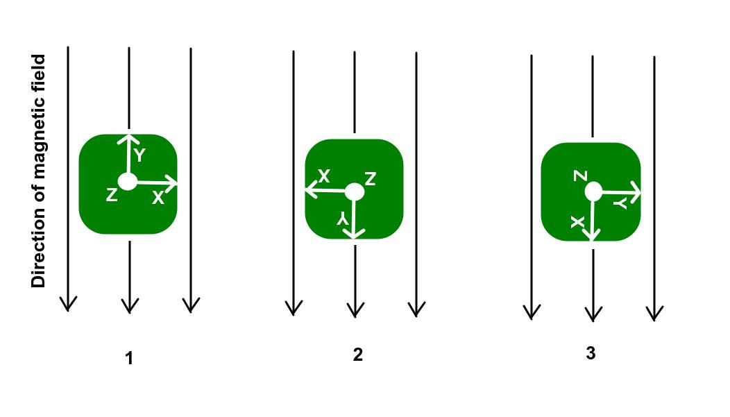
Let's call position one "straight ahead" and say that position 2 is rotated 180 degrees from position 1. In position 3 the sensor is rotated 90 degrees from position 1.

In positions 1 and 2, both X and Z would measure essentially zero since they are perpendicular to the field direction. The Y axes in both cases will measure the entire field strength but the signs will be opposite. In scenario 3, it is now X that measures the entire field strength while Y measures essentially zero.

As a level magnetometer is rotated, both the X and Y axes pass the same field in the same way. Because of this, we should expect the following of the X and Y data from a flat magnetometer that is rotated in a complete circle:

• The X and Y measurements should have the same minimum and maximum

• The measurements should cross zero twice per rotation

• The midpoint of the range of the measurements should be zero

• The measurements should be identical, but at different times during the rotation

Figure 3 shows a plot of magnetometer data as a sensor on a robot is rotated several times. The Y values in red mostly adhere to the above expectations, but the X values in blue deviate. The minimum and maximum are not equal and opposite, meaning that zero is not the midpoint. In fact, the X measurements remain below zero for the entire rotation, indicating a distortion along that axis. Fortunately, this is a distortion that can be measured and calibrated out.

Do I really need to calibrate if I don't need perfect accuracy?

If you rotate a sensor that is working properly the heading will cycle from -Pi to +Pi, crossing zero in the middle. There will be an abrupt jump as the heading goes from -Pi to +Pi or vice versa. This is normal, expected behavior.

Figure 4 shows the headings in blue that were calculated with the uncorrected data. The headings stay between 1 and 2 radians even though the sensor was being rotated in complete circles and should look more like the data in red. In short, I highly recommend you plan for regular calibration.

Calibration Procedure

Keep in mind that calibration needs to be done with the sensor mounted in its final position. You can calibrate it all by itself, but the correction values won't be correct once the distortions of the rest of a robot or whatever are then introduced. To calibrate the magnetometer, we need to follow these steps:

1. Either start recording all measurements or run a program that saves the highest and lowest values that occur for each axis

2. Rotate the sensor in one or more (preferably) complete circles about the z axis (

3. Note the highest and lowest values that occur for each axis

4. Find the midpoint of the range of values for each axis. For each axis, the midpoint = (min+max)/2

5. Record these midpoints to a file. - they are now the offsets we apply

6. Add a code to your heading calculation program to read the file and apply the offsets to each reading

In greater detail, let's look at each step:

Steps 1

Start your sensor streaming data and then your calibration program which, at this step, just needs to save every message to a vector. It is possible to do step 3 on this data live instead of saving it, but the latter gives you more opportunity to check the data for noise and outliers and apply some filter if necessary.

Step 2

Take your robot a flat, open spot outside and slowly rotate it a couple of times. The magnetometer I used is part of the IMU built into a ZED 2i stereo camera I had already mounted on a robot. I wrote a callback function for a ROS subscriber that simply appends each new value to a vector I could have either saved or used on the spot. This is the same data I shared in figure 3.

Step 3

Whether you read it from a file or just read it from the sensor, the goal is to find the lowest value and the highest value measured on each axis. You should end up with 2 variables for each axis.

Step 4

Find the midpoint of the range of values for each axis. For each axis, the midpoint = (min+max)/2

Step 5

Record these midpoints to a file so the heading calculator program can access them later.

Step 6

Apply to live data in your heading calculator program by subtracting the offsets from each and every raw measurement. The result should be data that adheres to the expectations we discussed earlier. Figure 5 shows my recorded data after calibration corrections have been made.

As you can see, the blue X and red Y data now have equal and opposite minimums and maximums and overall look very much the same. Figure 6 shows the result of performing the heading calculations we learned in the last article on this corrected data.

Now the calculated headings appropriately cover the expected range of -pi to +pi and matches our reference data quite accurately!

When to Recalibrate

Recalibration needs to be done when the magnetometer is moved to a different location on the robot (or whatever device you're using it in) or if there are changes to the robot that can affect the magnetic field (did you mount something else near the sensor?). It is also a good idea to recalibrate every few weeks or at least every couple of month, depending on the application's accuracy requirements. If you really need the best accuracy it only takes a minute to calibrate every day.

Let's get to the code

We need two programs: A program to find and save our calibration offsets, and a modified version of the heading calculator that applies the calibration offsets. Lets start with a simple calibration program that runs until 30 seconds has elapsed and some minimum number of samples have been collected. In practice, I prefer to have my program watch the data and look to confirm that 2-3 rotations have been completed.

C++

/******************************************************A sample program to collect and save calibration data*From the Practical Robotics blog at*www.lloydbrombach.com/blog**Lloyd Brombach*Feb 2023*******************************************************#include <iostream>#include <fstream>#include <vector>#include <chrono>#include <thread>using namespace std;double getRawDataX();double getRawDataY();int main(){    // vectors to store the readings until we are ready to save.    vector<double> xData;    vector<double> yData;    const int MIN_DATA_COUNT = 300;    const int ROTATION_TIME = 30; // 30 seconds for rotation    int time_elapsed = 0;    int last_time = time_elapsed;    // prompt the user to get ready to rotate the device    cout << "Get ready to rotate the device slowly for two complete rotations in " << ROTATION_TIME << " seconds\n";    cout << "to gather a minimum of " << MIN_DATA_COUNT << " samples. \n";    cout << "Press Enter when ready.\n";    cin.get();    // start collection    cout << "GO! " << ROTATION_TIME - time_elapsed << " seconds remaining. ";    auto start_time = chrono::steady_clock::now(); // start time    int samples = 0;                               // to count samples    // collect until time is up AND the minimum number of samples have been collected    while (time_elapsed < ROTATION_TIME || samples < MIN_DATA_COUNT)    {        // get the magnetometer data and save it in the vector        xData.push_back(getRawDataX());        yData.push_back(getRawDataY());        // give a progress update every second        if (last_time != time_elapsed)        {            cout << "\n"                 << ROTATION_TIME - time_elapsed << " seconds remaining. " << samples << " samples collected.";            last_time = time_elapsed;        }        this_thread::sleep_for(chrono::milliseconds(100)); // wait for 0.1 seconds        time_elapsed = chrono::duration_cast<chrono::seconds>(chrono::steady_clock::now() - start_time).count();        samples++; // update count    }    // write the collected data to file and find the min and max values    ofstream outFile("raw_data.dat");    double minX = xData[0], maxX = xData[0];    double minY = yData[0], maxY = yData[0];    for (int i = 0; i < xData.size(); i++)    {        outFile << xData[i] << " " << yData[i] << endl;        // find min and max for each vector        if (xData[i] < minX)            minX = xData[i];        if (xData[i] > maxX)            maxX = xData[i];        if (yData[i] < minY)            minY = yData[i];        if (yData[i] > maxY)            maxY = yData[i];    }    outFile.close();    cout << endl         << "Data collection complete. Saved " << samples << " measurements" << endl;    // calculate midpoint of min and max for each vector    double midX = (minX + maxX) / 2.0;    double midY = (minY + maxY) / 2.0;    // write midpoint values to calibration file    ofstream calibFile("calibration_data.txt");    calibFile << midX << " " << midY << endl;    calibFile.close();    cout << "\nCalibration data saved." << endl;        return 0;}double getRawDataX(){    // replace with code to fetch and return your actual data    return rand();}double getRawDataY(){    // replace with code to fetch and return your actual data    return rand();}

With the calibration offsets saved to a file, your compass heading calculation program just needs a function to retrieve those values and to subtract those values from the raw data as it comes in.

double offset_x, offset_y; // global variables to store offsetsvoid read_calibration_data() {    ifstream calibFile("calibration_data.txt");    calibFile >> offset_x >> offset_y;    calibFile.close();}

Then it's as simple as subtracting those values from the raw measurements:

double corrected_x =  getRawDataX() - offset_x;double corrected_y =  getRawDataY() - offset_Y;

Python

#######################################################A sample program to collect and save calibration data#From the Practical Robotics blog at#www.lloydbrombach.com/blog##Lloyd Brombach#Feb 2023######################################################import timeimport randomdef get_raw_data_x():    # replace with code to fetch and return your actual data    return random.random()def get_raw_data_y():    # replace with code to fetch and return your actual data    return random.random()# vectors to store the readings until we are ready to save.x_data = []y_data = []MIN_DATA_COUNT = 300ROTATION_TIME = 30  # 30 seconds for rotationtime_elapsed = 0last_time = time_elapsed# prompt the user to get ready to rotate the deviceprint(f"Get ready to rotate the device slowly for two complete rotations in {ROTATION_TIME} seconds")print(f"to gather a minimum of {MIN_DATA_COUNT} samples.")input("Press Enter when ready.\n")# start collectionprint(f"GO! {ROTATION_TIME - time_elapsed} seconds remaining. ")start_time = time.monotonic() # start timesamples = 0 # to count samples# collect until time is up AND the minimum number of samples have been collectedwhile time_elapsed < ROTATION_TIME or samples < MIN_DATA_COUNT:    # get the magnetometer data and save it in the vector    x_data.append(get_raw_data_x())    y_data.append(get_raw_data_y())    # give a progress update every second    if last_time != time_elapsed:        print(f"\n{ROTATION_TIME - time_elapsed} seconds remaining. {samples} samples collected.", end="")        last_time = time_elapsed    time.sleep(0.1) # wait for 0.1 seconds    time_elapsed = int(time.monotonic() - start_time)    samples += 1 # update count# write the collected data to file and find the min and max valueswith open("raw_data.dat", "w") as outFile:    minX, maxX = x_data[0], x_data[0]    minY, maxY = y_data[0], y_data[0]    for i in range(len(x_data)):        outFile.write(str(x_data[i]) + " " + str(y_data[i]) + "\n")        # find min and max for each vector        if x_data[i] < minX:            minX = x_data[i]        if x_data[i] > maxX:            maxX = x_data[i]        if y_data[i] < minY:            minY = y_data[i]        if y_data[i] > maxY:            maxY = y_data[i]    outFile.close()    print("\nData collection complete. Saved", len(x_data), "measurements")    # calculate midpoint of min and max for each vector    midX = (minX + maxX) / 2.0    midY = (minY + maxY) / 2.0    # write midpoint values to calibration file    with open("calibration_data.txt", "w") as calibFile:        calibFile.write(str(midX) + " " + str(midY) + "\n")        calibFile.close()        print("Calibration data saved.")

With the calibration offsets saved to a file, your compass heading calculation program just needs a function to retrieve those values and to subtract those values from the raw data as it comes in.

offset_x = 0.0offset_y = 0.0def read_calibration_data():    global offset_x, offset_y    with open("calibration_data.txt", "r") as calibFile:        offset_x, offset_y = map(float, calibFile.readline().split())    print("Calibration data read.")

Then it's as simple as subtracting those values from the raw measurements:

corrected_x =  getRawDataX() - offset_xcorrected_y =  getRawDataY() - offset_Y

MATLAB

%%%%%%%%%%%%%%%%%%%%%%%%%%%%%%%%%%%%%%%%%%%%%%%%%%%%%%%A sample program to collect and save calibration data%From the Practical Robotics blog at%www.lloydbrombach.com/blog%%Lloyd Brombach%Feb 2023%%%%%%%%%%%%%%%%%%%%%%%%%%%%%%%%%%%%%%%%%%%%%%%%%%%%%%function main()    % vectors to store the readings until we are ready to save.    x_data = [];    y_data = [];    MIN_DATA_COUNT = 300;    ROTATION_TIME = 30; % 30 seconds for rotation    time_elapsed = 0;    last_time = time_elapsed;    % prompt the user to get ready to rotate the device    disp(['Get ready to rotate the device slowly for two complete rotations in ' num2str(ROTATION_TIME) ' seconds']);    disp(['to gather a minimum of ' num2str(MIN_DATA_COUNT) ' samples.']);    input('Press Enter when ready.\n', 's');    % start collection    disp(['GO! ' num2str(floor(ROTATION_TIME - time_elapsed)) ' seconds remaining. ']);    start_time = tic; % start time    samples = 0; % to count samples    % collect until time is up AND the minimum number of samples have been collected    while time_elapsed < ROTATION_TIME || samples < MIN_DATA_COUNT        % get the magnetometer data and save it in the vector        x_data(end+1) = getRawDataX();        y_data(end+1) = getRawDataY();        % give a progress update every second        if time_elapsed - last_time >= 1            disp([num2str(floor(ROTATION_TIME - time_elapsed)) ' seconds remaining. ' num2str(samples) ' samples collected.']);            last_time = time_elapsed;        end        pause(0.1); % wait for 0.1 seconds        time_elapsed = toc(start_time);        samples = samples + 1; % update count    end    minX = x_data(1);    maxX = x_data(1);    minY = y_data(1);    maxY = y_data(1);for i = 1:samples    % find min and max for each vector    if x_data(i) < minX        minX = x_data(i);    end    if x_data(i) > maxX        maxX = x_data(i);    end    if y_data(i) < minY        minY = y_data(i);    end    if y_data(i) > maxY        maxY = y_data(i);    endend% calculate midpoint of min and max for each vectormidX = (minX + maxX) / 2.0;midY = (minY + maxY) / 2.0;% save the data to a .mat filesave('raw_data.mat', 'x_data', 'y_data');disp(['Data collection complete. Saved ' num2str(samples)]);% save midpoint values to calibration filesave('calibration_data.mat', 'midX', 'midY'); disp('Calibration data saved.');endfunction x = getRawDataX()    % replace with code to fetch and return your actual data    x = rand();endfunction y = getRawDataY()    % replace with code to fetch and return your actual data    y = rand();end

With the calibration offsets saved to a file, your compass heading calculation program just needs a function to retrieve those values and to subtract those values from the raw data as it comes in. MATLAB makes this ridiculously easy.

function [offset_x, offset_y] = read_calibration_data()    % Load calibration data from .mat file    load('calibration_data.mat', 'offset_x', 'offset_y');end

Then it's as simple as subtracting those values from the raw measurements:

corrected_x =  getRawDataX() - offset_x;corrected_y =  getRawDataY() - offset_Y;

Conclusion

With parts 1 and 2 in this series behind us, we can now calculate accurate headings even when the magnetic field measurements are corrupted by nearby disturbances, but there is one more factor that can ruin our calculations – tilt. If the sensor is not fairly level, the X and Y measurements cannot be trusted. In the next article in this series, I willattempt to explain why and what we can do about it.

Compass headings can be essential for many autonomous mobile robots, and magnetometers such as those included in the popular LSM303, MPU-6050, and BNo055 Inertial Measurement Units (IMUs) are commonly used for this task. Magnetometers are sometimes called a digital compass, but this is a bit misleading as there is more to it than that. This article aims to help you get the function of a digital compass out of a plain old magnetometer.

Magnetometers measure the Earth's magnetic field, allowing us to calculate a compass heading for our mobile robots or other applications based on these measurements. This article assumes you have the sensor data and just need to calculate headings with it. If you aren't quite there yet or want to learn more, my book, "Practical Robotics in C++," provides an in-depth guide to working with sensors, including sample programs. You can also find sensor and serial data tutorials at the Practical Robotics YouTube channel.

Products Mentioned in this article:

LSM303 Inertial Measurement Unit

MPU-6050 Inertial Measurement Unit

BNo055 Absolute Orientation Sensor

Practical Robotics in C++

Disclaimer: Please note that the products linked on this page are not sponsored, but as an Amazon Associate I earn from qualifying purchases.

While the math to get a heading from raw magnetometer data is straightforward, there are some variations for many applications that makes it impossible to give a simple formula or chunk of code and send you on your way. Generally, though, these are the steps to calculate a heading:

• Get magnetometer data for at least the X and Y axes

• Maybe negate the Y value, maybe not

• Use trig to calculate the direction of the magnetic field vector

• Apply a correction to align with your coordinate convention

• Compensate for magnetic declination

We'll talk about each of these steps in this article and add a couple more in the future to compensate for less than perfect conditions.

Some Background Info

The true north and south poles refer to the geographic points located at the top and bottom of the earth's rotational axis, respectively. These points mark the earth's axis of rotation and are used as a reference point for navigation and mapping purposes. On the other hand, the magnetic north and south poles are determined by the Earth's magnetic field, which is generated by the movement of molten iron in the planet's core. The magnetic north and south poles are not located at the same place as the true north and south poles. In fact, the Earth's magnetic north pole is currently located in northern Canada, while the magnetic south pole is located off the coast of Antarctica. Lastly, it's worth noting that what is commonly referred to as magnetic north is actually the location of the earth's magnetic south pole. This can be a bit confusing, but it's because the Earth's magnetic field lines emerge from the magnetic south pole and converge at the magnetic north pole. Figure 1 is my attempt at illustrating this stuff.

Magnetometers measure the strength of the magnetic field, and we can determine the direction of the field if we measure in the X, Y, and Z axes at once (most magnetometers do this). For heading, we are concerned with the direction of the horizontal component of that direction, so we will start with using just the X and Y measurements. This works fine if the sensor is more or less level, but we will need to build on this method and include Z data later on to compensate for tilt. Figure 2 shows a magnetometer placed with its y-axis aligned with the Earth's magnetic field.

The strength of the field on the x-axis is nearly zero because it is perpendicular to the field, and the strength of the field in the y-direction is either at its maximum or minimum (depending on whether it's facing North or South and how near or far you are from the poles). Whether the reading is positive or negative, we can say that the absolute value of the y measurement is at its maximum.

If the sensor is rotated so the x-axis is pointing north, the absolute value of x-axis measurement will increase to the same value and the absolute value of y-axis measurement will decrease until it reaches zero. If the wording above feels clunky or unclear, just takeaway three key things:

• As it the sensor rotates, the strength of the field is always increasing on one axis and decreasing on the other.

• The measurement will be essentially zero for an axis facing East or West. ("Essentially" because we must expect sensor noise and imperfections)

• The measurement will be at its maximum absolute value for an axis that is facing North or South. The value will be equal but opposite facing the opposite direction.

Thanks to these predictable characteristics, we can easily use the trigonometry arctangent function to calculate the angle between the sensor's axes and the earth's magnetic field. Without further delay, lets dive into why you really came here and work the steps I listed above.

Get Magnetometer Data

As I mentioned earlier, getting data from your sensor is outside the scope of this article. The rest of this article assumes you have readings called X, Y, and Z. Your sensor might return values in either Tesla or Gauss, but because the calculations rely on the ratios and not the absolute values it does not matter which for our purposes. I will note that ROS convention is to use Tesla.

Maybe Negate the Y Value or Maybe Not

The direction of the earth's magnetic field can sometimes be significantly vertical and even cause a Y value to read negative when the sensor is pointed north (or tilted just little). The same sensor further south could read a positive value when pointed north. I have so far not found a definitive resource or map that indicates in a simple way where a person might need to negate that Y value, but I have found that Michigan, USA is far enough north and in a region where it is necessary. The best advice I have is to complete the calculations without negating Y, then do some tests. Heading values should increase when turning the sensor counter clockwise and decrease when turning clockwise. If this is not the case, try negating Y for the arctangent step below.

Arctangent: atan() vs atan2()

Most programming languages I've used have two arctangent functions we can use to calculate the angle between the x axis of the magnetometer and magnetic South. The first is atan(y/x), which only takes one argument (y/x is just a single value) and can only give a result in the first or fourth quadrant of the unit circle (from -pi/2 to pi/2). This requires extra code to determine the correct quadrant and heading so I suggest using atan2(y, x) as it uses y and x separately to calculate for all four quadrants, providing a result between -pi and pi. Quite simply, let's use:

magneticHeading = atan2(Y, X)//ormagneticHeading = atan2(-Y, X)

Note that the parameter order for atan2 is y before x every programming languag I've used it in (C++, Java, Matlab, and Python). Also don't forget that we use radians instead of degrees in robotics and trigonometry, but they can be easily converted using the formula degrees = radians * (180/pi) if needed.

Apply a correction to align with your coordinate convention

The result from the atan2() function is an angle between the magnetic field lines and the x axis of the magnetometer. However, to use this angle as a compass heading in a specific application, we need to adjust it to match the convention used by that application. For example, in ROS (Robot Operating System), the convention for compass headings is to use an angle between the positive y-axis and the direction of magnetic North. To convert the angle from atan2() to this convention, we need to add 90 degrees (or pi/2 radians) to the result.

magneticHeading += M_PI / 2 

Now we just need to ensure that the result stays within the bounds of -PI to +PI:

while (magneticHeading > M_PI)     magneticHeading -= 2 * M_PIwhile (magneticHeading <= -M_PI)     magneticHeading += 2 * M_PI

Compensate for magnetic declination

There is a difference between the magnetic axis of the Earth and it's axis of rotation. Maps typically adhere to rotational axis the truth, but our calculations so far are relative to the magnetic axis. The difference is measured as a declination angle, which varies in different parts of the world. In Detroit, Michigan the declination is about -8 degrees or -0.139 radians. We simply add this to our calculated magnetic heading to align with the Earth's rotational axis and thus, with most maps, GPS coordinates, etc.

declination = -0.139trueHeading = magneticHeading + declination

Declination varies a LOT just around the United States, so be sure to ask Google for the declination value for your location. It's probably in degrees so don't forget to convert it to radians.

Putting it all together: The C++, Python, and MATLAB code

All of my rambling on so far can be summarized with this formula:

heading = magnetic_field_direction + convention_offset + declination

Assuming you already have variables called X and Y populated with magnetometer data, the following code blocks put it together:

C++

#include <iostream>#include <cmath>//radians. Location specific.double declination = -0.139;// adjustment needed for ROS conventiondouble convention_offset = -1.57;// calculate magnetic field directiondouble magnetic_field_direction = atan2(-Y, X);// calculate true headingdouble trueHeading = magnetic_field_direction + convention_offset + declination;// ensure result is in bounds of -PI to +PIwhile (trueHeading < -M_PI)     trueHeading += 2.0 * M_PI;while (trueHeading > M_PI)    trueHeading -= 2.0 * M_PI;

Python

import math# radians. Location specific.declination = -0.139# adjustment needed for ROS conventionconvention_offset = -1.57# calculate magnetic field direction. Negate Y if necessarymagnetic_field_direction = math.atan2(Y, X)# calculate true headingtrueHeading = magnetic_field_direction + convention_offset + declination# ensure result is in bounds of -PI to +PItrueHeading = (trueHeading + math.pi) % (2*math.pi) - math.pi

MATLAB

% radians. Location specific.declination       = -0.139% adjustment needed for ROS conventionconvention_offset = -1.57% calculate magnetic field direction. Negate Y if necessarymagnetic_field_direction = atan2(Y, X)% calculate true headingtrueHeading = magnetic_field_direction + convention_offset + declination% ensure result is in bounds of -PI to +PItrueHeading = wrapToPi(trueHeading);

Why are my headings incorrect?

Compass headings can be calculated using magnetometer data, but it is important to note that the data may be distorted by nearby magnets or iron objects, as well as the sensor itself. If the disturbance is fixed in relation to the sensor (like parts of the robot itself), calibration can be used to measure and cancel out the effect. I will show you how to easily do this in my very next article, again in C++, Python, and MATLAB.

It is also important to know that the result is only reliable if the sensor is relatively flat. Compensating for tilt will be the topic of the final article in this series.

Peace out

I hope you found this article helpful in calculating compass headings using magnetometers. Remember, while the math may seem straightforward, there are variations and nuances to consider based on your application. Don't hesitate to seek additional resources such as our book "Practical Robotics in C++" and tutorials on the Practical Robotics YouTube channel. Thanks for reading and keep exploring and experimenting to optimize your robot's navigation!