自动驾驶高精度地图文件格式(Opendrive、Lanelet2、VectorMap)
常用的高精度地图格式:
1、Opendrive
百度Apollo也采用这种格式
2、Lanelet2
C++实现的高精度地图库:https://github.com/fzi-forschungszentrum-informatik/lanelet2
3、VectorMap
矢量地图
常用的高精度地图格式:
1、Opendrive
百度Apollo也采用这种格式
2、Lanelet2
C++实现的高精度地图库:https://github.com/fzi-forschungszentrum-informatik/lanelet2
3、VectorMap
矢量地图
高精地图即为“两高一多”的地图,在自动驾驶中常常被称为HapMap,这是自动驾驶汽车中非常重要的一部分


高精地图是一种语义地图,概括地说,就是利用SLAM/SFM等算法融合多种传感器数据,构建高精度的 三维点云地图,在点云地图上或者是图像上,对所用到的元素进行分类和提取、之后对不同元素分别进行矢量化并构建路网与车道关联关系,最后进行质量校验,形 成一套地图引擎来存储并支撑其他模块的需求。
高精地图制作完成后,其数据量其实是非常小的。地图数据可以存储在云端,也 可以直接直接在本地,大地图还有可以用数据库来存储。先暂且不论地图格式是Lanelet2还是OpenDrive以及其他,完整的理解高精地图的元素结 构设计,以及数据存储和使用则为重中之重,后续的自定义格式要求可按自己的需求来适配。
对于3km以内的小地图而言,一般可以采取手工标注点云地图的方法来制图。目前我了解到的以下软件均可,比如
Autocore MapToolBox插件

构建点云地图可以用一些主流的激光SLAM算法,结合多种传感器来完成,其中要保证户外场景的建图效果,IMU和GPS是必须的,下面有一些推荐的开源算法,按优先级排列

自动标注涉及到的算法相当多,流程大致如下:

对比下来发现采用Autoware的地图标注插件更好,Unity + MapToolBox进行标注,插件地址如下:https://github.com/autocore-ai/MapToolbox,这里注意下载的Unity版本需2019.3+,在Windows环境下使用,最新版的priview6已经加入对road mark和crosswalk的支持。目前Autoware社区已经增加了对Lanelet2的支持。

Apollo Opendrive高精地图的话一般存在下面四种思路。


由 于目前支撑Opendrive的开源lib库很少,虽然自己写也不是特别费劲,可以利用其他的开源地图框架,生成高精地图之后再转换为Apollo Opendrive格式。这里目前可选择的仅仅是Liblanelets/Lanlets2,按照Lanlets2的接口规范可以生成OSM地图,在用开 源的JSOM编辑器编辑完OSM地图后,再 转换成Apollo Opendrive地图

地图格式官方推荐的是OSM格式(XML),开源可编辑。当然也可以是二进制文件,加载速度快,缺点是不可直接编辑。下面的地图文件是按XML形式来存储的,结构十分明朗。关于OSM规范,可以参考其WIKI,https://wiki.openstreetmap.org/wiki/Map_Features。

地图里面的每一个3D点都会用一个node标签存储,包含其经纬度LaLon,id是其唯一标志。后续的way标签存储lineString形式的元素,通过id引用node节点存储的3D点。而和交规相关的relation标签则又引用这些way id。


我们在JOSM编辑器中打开可以看到地图的基本形状,此编辑器的使用方法可查看官网https://learnosm.org/en/josm/correcting-imagery-offset/。
下图是一个复杂的十字路口,地图上所有的黄色小框框都是一个3D/2D坐标点。这里红色的线是地图里面的stop_line,在软件界面右侧可以看到其属性是stop line,并且有四个节点。地图上画出来了所有的车道线,路沿,人行横道,绿化带区域等,还有各个road user(比如行人,车辆等)需要遵守的交通规则,以及车辆在十字路口可能的换道路线(现实中是没有的,属性定义为virtual)。


Lanelet2代码的安装可以参考官方文档https://github.com/JokerJohn/Lanelet2,其层级结构如下

我们常用的代码在lanelet_core、lanelet_io、lanelet_projection、lanelet_routing和lanelet_traffic_rules这几个模块中。项目采用gtest框架来测试,阅读起来比较容易。


| Indicator |
Description |
| 0 |
Fix not available or invalid |
| 1 |
Single point |
| Converging PPP (TerraStar-L) |
|
| 2 |
Pseudorange differential |
| Converged PPP (TerraStar-L) |
|
| Converging PPP (TerraStar-C PRO, TerraStar-X) |
|
| 4 |
RTK fixed ambiguity solution |
| 5 |
RTK floating ambiguity solution |
| Converged PPP (TerraStar-C PRO, TerraStar-X) |
|
| 6 |
Dead reckoning mode |
| 7 |
Manual input mode (fixed position) |
| 8 |
Simulator mode |
| 9 |
WAAS (SBAS)1 |
Field |
Structure |
Description |
Symbol |
Example |
| 1 |
$GPGGA |
Log header |
|
$GPGGA |
| 2 |
utc |
UTC time status of position (hours/minutes/seconds/ decimal seconds) |
hhmmss.ss |
202134.00 |
| 3 |
lat |
Latitude (DDmm.mm) |
llll.ll |
5106.9847 |
| 4 |
lat dir |
Latitude direction (N = North, S = South) |
a |
N |
| 5 |
lon |
Longitude (DDDmm.mm) |
yyyyy.yy |
11402.2986 |
| 6 |
lon dir |
Longitude direction (E = East, W = West) |
a |
W |
| 7 |
quality |
refer to Table: GPS Quality Indicators |
x |
1 |
| 8 |
# sats |
Number of satellites in use. May be different to the number in view |
xx |
10 |
| 9 |
hdop |
Horizontal dilution of precision |
x.x |
1.0 |
| 10 |
alt |
Antenna altitude above/below mean sea level |
x.x |
1062.22 |
| 11 |
a-units |
Units of antenna altitude (M = metres) |
M |
M |
| 12 |
undulation |
Undulation - the relationship between the geoid and the WGS84 ellipsoid |
x.x |
-16.271 |
| 13 |
u-units |
Units of undulation (M = metres) |
M |
M |
| 14 |
age |
Age of correction data (in seconds) The maximum age reported here is limited to 99 seconds. |
xx |
(empty when no differential data is present) |
| 15 |
stn ID |
Differential base station ID |
xxxx |
(empty when no differential data is present) |
| 16 |
*xx |
Check sum |
*hh |
*48 |
| 17 |
[CR][LF] |
Sentence terminator |
|
[CR][LF] |
1: URL
https://ww2.mathworks.cn/help/fusion/ug/tuning-kalman-filter-to-improve-state-estimation.html
This example shows how to tune process noise and measurement noise of a constant velocity Kalman filter.
此示例显示如何调整恒速卡尔曼滤波器的过程噪声和测量噪声。
This example explores one of the simplest motion models: a constant velocity motion model in two dimensions. A constant velocity motion model assumes that the object moves with a nearly constant velocity. The state vector consists of four parameters that represent the position and velocity in the x- and y- dimensions.
这个例子探讨了最简单的运动模型之一:二维的匀速运动模型。匀速运动模型假定物体以几乎恒定的速度运动。状态向量由四个参数组成,分别表示x维和y维的位置和速度。
There are other popular motion models, for example a constant turn that assumes the object moves mostly along a circular arc with a constant speed. More complicated models, such as constant acceleration, help when an object moves for a significant duration of time according to the model. Nonetheless, a very simple motion model like the constant velocity model can be used successfully to track an object that gradually changes its direction or speed over time. A Kalman filter achieves this flexibility by providing an additional parameter called process noise.
还有其他流行的运动模型,例如,假设物体以恒定速度沿着圆弧运动的恒定转弯。更复杂的模型,如恒定加速度,当一个物体根据模型移动了很长一段时间时,就会有所帮助。尽管如此,一个非常简单的运动模型,如恒定速度模型,可以成功地用于跟踪一个随着时间逐渐改变其方向或速度的物体。卡尔曼滤波器通过提供一个称为过程噪声的附加参数来实现这种灵活性。
In reality, objects do not exactly follow a particular motion model. Therefore, when a Kalman filter estimates the motion of an object, it must account for unknown deviations from the motion model. The term ‘process noise’ is used to describe the amount of deviation, or uncertainty, of the true motion of the object from the chosen motion model. Without process noise, a Kalman filter with a constant velocity motion model fits a single straight line to all the measurements. With process noise, a Kalman filter can give newer measurements greater weight than older measurements, allowing for a change in direction or speed. While 'noise' and 'uncertainty' are terms that connote the idea of a chaotic deviation from the model, process noise can also allow for small, predictable, changes to the true motion of an object that would otherwise require considerably more complex motion models.
在现实中,物体并不完全遵循特定的运动模型。因此,当卡尔曼滤波器估计一个物体的运动时,它必须考虑到运动模型的未知偏差。术语“过程噪声”用于描述对象的真实运动与所选运动模型的偏差量或不确定性。在没有过程噪声的情况下,具有匀速运动模型的卡尔曼滤波器将一条直线拟合到所有测量值上。对于过程噪声,卡尔曼滤波器可以给予新的测量比旧的测量更大的权重,允许方向或速度的改变。虽然“噪声”和“不确定性”是包含混沌偏离模型的概念的术语,但过程噪声也可以允许对物体的真实运动进行小的、可预测的变化,否则这些变化将需要相当复杂的运动模型。
This example shows a car moving along a curving road with a relatively constant speed profile and uses a constant velocity motion model with a small amount of process noise to account for the minor deviations due to changes in steering and speed. Process noise allows the filter to account for small changes in speed or direction without estimating how fast the car is accelerating or turning. If you examine the trajectory of a car over a short duration of time, you may observe that it goes nearly straight. It is only over larger durations of time that you can observe the change in the direction of motion of the car.
这个例子展示了一辆汽车以相对恒定的速度沿着弯曲的道路行驶,并使用恒定速度运动模型和少量的过程噪声来解释由于转向和速度变化而产生的微小偏差。过程噪声允许过滤器解释速度或方向的微小变化,而无需估计汽车加速或转弯的速度有多快。如果你在短时间内观察一辆汽车的轨迹,你可能会观察到它几乎是直线行驶的。只有在更长的时间内,你才能观察到汽车运动方向的变化。
Process noise has an inherent tradeoff. A low process noise may cause the filter to ignore rapid deviations from the true trajectory and instead favor the motion model. This limits the amount of deviation from the motion model that the true trajectory can have at any particular time. A high process noise admits greater local deviations from the motion model but makes the filter too sensitive to noisy measurements.
过程噪声有一个内在的权衡。低过程噪声可能导致滤波器忽略快速偏离真实轨迹,而倾向于运动模型。这限制了真实轨迹在任何特定时间与运动模型的偏差。一个高的过程噪声允许更大的局部偏离运动模型,但使滤波器对噪声测量过于敏感。
Kalman filters also model "measurement noise" which helps inform the filter how much it should weight the new measurements versus the current motion model. Specifying a high measurement noise indicates that the measurements are inaccurate and causes the filter to favor the existing motion model and react more slowly to deviations from the motion model.
卡尔曼滤波器还对“测量噪声”进行建模,这有助于告知滤波器应该对新测量值和当前运动模型进行多大的加权。指定高测量噪声表示测量不准确,并导致滤波器倾向于现有的运动模型,并且对运动模型的偏差反应更慢。
The ratio between the process noise and the measurement noise determines whether the filter follows closer to the motion model, if the process noise is smaller, or closer to the measurements, if the measurement noise is smaller.
过程噪声与测量噪声之间的比率决定了如果过程噪声较小,滤波器是更接近运动模型,或者如果测量噪声较小,滤波器更接近测量值。
A constant velocity filter tuned to follow an object that has a steady speed and turns very slowly over a long distance, may not work as well when estimating an object that slows down or turns quickly. Therefore, it is important to tune the filter for the entire range of motion types you expect it to filter. It is also important to consider the expected amount of measurement noise. If you tune the filter using low-noise measurements, the filter may track changes in the motion model better. However, if you use the same tuned filter to track an object measured in a higher noise environment, the resulting track may be unduly influenced by outliers.
一个恒速滤波器被调整为跟踪一个具有稳定速度并且在很长一段距离内旋转非常缓慢的物体,可能在估计一个减速或快速旋转的物体时效果不佳。因此,重要的是要调整过滤器的整个范围的运动类型,你希望它过滤。考虑测量噪声的预期量也很重要。如果您使用低噪声测量来调整滤波器,则滤波器可以更好地跟踪运动模型中的变化。但是,如果使用相同的调谐滤波器来跟踪在较高噪声环境中测量的对象,则产生的跟踪可能会受到异常值的过度影响。
The following code generates a training trajectory that models the path of a vehicle travelling at 30 m/s on a highway. It also generates a test trajectory for a vehicle that has a similar speed and follows a highway of similar curvature variation.
下面的代码生成了一个训练轨迹,该轨迹模拟了在高速公路上以30米/秒的速度行驶的车辆的路径。它还为具有相似速度并沿着相似曲率变化的高速公路行驶的车辆生成测试轨迹。
% Specify the training trajectorytrajectoryTrain = waypointTrajectory( ... [96.4 159.2 0; 2047 197 0;2245 -248 0; 2407 -927 0], ... [0; 71; 87; 110], ... 'GroundSpeed', [30; 30; 30; 30], ... 'SampleRate', 2);dtTrain = 1/trajectoryTrain.SampleRate;timeTrain = (0:dtTrain:trajectoryTrain.TimeOfArrival(end));[posTrain, ~, velTrain] = lookupPose(trajectoryTrain,timeTrain);% Specify the test trajectorytrajectoryTest = waypointTrajectory( ... [-2.3 72 0; -137 -204 0; -572 -937 0; -804 -1053 0; -887 -1349 0; ... -674 -1608 0; 368 -1604 0; 730 -1599 0; 1633 -1581 0; 1742 -1586 0], ... [0; 8; 34; 42; 53; 64; 97; 107; 133; 136], ... 'GroundSpeed', [35; 35; 34; 30; 30; 30; 35; 35; 35; 35], ... 'SampleRate', 2);dtTest = 1/trajectoryTest.SampleRate;timeTest = (0:dtTest:trajectoryTest.TimeOfArrival(end));[posTest, ~, velTest] = lookupPose(trajectoryTest,timeTest);% Plot the trajectoriesfigureplot(posTrain(:,1),posTrain(:,2),'.', ... posTest(:,1), posTest(:,2),'.');axis equal;grid on;legend('Training','Test');xlabel('X Position (m)');ylabel('Y Position (m)');title('True Position')
![]()
As stated above, create a Kalman Filter to use a two-dimensional motion model.
KF = trackingKF('MotionModel','2D Constant Velocity')
KF = trackingKF with properties: State: [4x1 double] StateCovariance: [4x4 double] MotionModel: '2D Constant Velocity' ProcessNoise: [2x2 double] MeasurementModel: [2x4 double] MeasurementNoise: [2x2 double] MaxNumOOSMSteps: 0 EnableSmoothing: 0
This example contains position-only measurements of the vehicles. The constant velocity motion model, '2D Constant Velocity', has a state vector of the form: [px; vx; py; vy], where px and py are the positions in the x- and y-directions, respectively; and vx and vy are the velocities in the x- and y-directions, respectively.
trueStateTrain = [posTrain(:,1), velTrain(:,1), posTrain(:,2), velTrain(:,2)]';trueStateTest = [posTest(:,1), velTest(:,1), posTest(:,2), velTest(:,2)]';
Since the truth is known for both the training and test data, you can directly simulate measurements. You obtain the position measurement by pre-multiplying the state vector by the MeasurementModel property of the filter. The MeasurementModel property, specified as the matrix, [1 0 0 0; 0 0 1 0], corresponds to position-only measurements. You also add measurement noise to these position measurements.
s = rng;rng(2021);posSelector = KF.MeasurementModel; % Position from statermsSensorNoise = 5; % RMS deviation of sensor data noise [m]% Training Data - Normal Sensor. Position OnlytruePosTrain = posSelector * trueStateTrain;measPosTrain = truePosTrain + rmsSensorNoise * randn(size(truePosTrain))/sqrt(2);% Test Data - Normal Sensor. Position OnlytruePosTest = posSelector * trueStateTest;measPosTest = truePosTest + rmsSensorNoise * randn(size(truePosTest))/sqrt(2);
Now the filter can be constructed and tuned using the training data and evaluated using the test data.
A simple way to initialize the state vector is to use the first position measurement and approximate the velocity using the first two measurements.
initStateTrain([1 3]) = measPosTrain(:,1);initStateTrain([2 4]) = (measPosTrain(:,2) - measPosTrain(:,1))./dtTrain;initStateTest([1 3]) = measPosTest(:,1);initStateTest([2 4]) = (measPosTest(:,2) - measPosTest(:,1))./dtTest;
The state covariance matrix should also be initialized to account for the uncertainty in measurement. To start, initialize just the main diagonal viadiag[σPxσVxσPyσVz]and adjust the position terms to correspond to the noise of the sensor. The velocity terms have higher noise since they are based on two measurements of position, not one.
initStateCov = diag(([1 2 1 2]*rmsSensorNoise.^2));
Process noise can be estimated via the expected deviation from constant velocity using a mean squared step change in velocity at each time step. Using the scalar form for process noise ensures that the components in the x- or y- directions are treated equally.
Qinit = var(vecnorm(diff(velTrain)./dtTrain,2,1))
Qinit = 15.2404
For many sensors, measurement noise is a known quantity often measured with an RMS value. Initialize the covariance to the square of this value.
Rinit = rmsSensorNoise.^2
Rinit = 25
Now you can set the process noise and measurement noise on the filter object.
KF.ProcessNoise = Qinit;KF.MeasurementNoise = Rinit;
The helper function, evaluateFilter sets up the filter and computes the RMS error of the predicted position against the true position of the training set:
errorTunedTrain = evaluateFilter(KF, initStateTrain, initStateCov, posSelector, dtTrain, measPosTrain, truePosTrain)
errorTunedTrain = 2.9624
Compare the filtered position error against the uncorrected raw measurements of the training set:
rms(vecnorm(measPosTrain - truePosTrain,2,1))
ans = 4.7319
It is clear that the filter obtained a much better position estimate.
In the test trajectory, the vehicle turns a little bit more and has a few acceleration changes. Therefore, it is expected that the filter estimate may not be as good as that of the training trajectory.
errorTunedTest = evaluateFilter(KF, initStateTest, initStateCov, posSelector, dtTest, measPosTest, truePosTest)
errorTunedTest = 3.7157
Nevertheless, it still is better than just using the raw measurements alone.
rms(vecnorm(measPosTest - truePosTest,2,1))
ans = 5.2553
You can sweep through a few process noise values and determine a desirable value for both the training and test cases.
nSweep = 100;Qsweep = linspace(1,50,nSweep);errorTunedTrain = zeros(1,nSweep);errorTunedTest = zeros(1,nSweep);for i = 1:nSweep KF.ProcessNoise = Qsweep(i); errorTunedTrain(i) = evaluateFilter(KF, initStateTrain, initStateCov, posSelector, dtTrain, measPosTrain, truePosTrain); errorTunedTest(i) = evaluateFilter(KF, initStateTest, initStateCov, posSelector, dtTest, measPosTest, truePosTest);endplot(Qsweep,errorTunedTrain,'-',Qsweep,errorTunedTest,'-');legend("training","test")xlabel("Process Noise (Q)")ylabel("RMS position error");
![]()
As seen in the above plot and in the code below, the training set has a local minimum when setting Q to 5.4 for the training set, and 13 for the test set.
[minErrorTunedTrain, iMinTrain] = min(errorTunedTrain);[minErrorTunedTest, iMinTest] = min(errorTunedTest);minErrorTunedTrain
minErrorTunedTrain = 2.8540
Qsweep(iMinTrain)
ans = 5.4545
minErrorTunedTest
minErrorTunedTest = 3.7141
Qsweep(iMinTest)
ans = 13.8687
Variations in the optimal point are expected and are due to the differences in the trajectories. With a small amount of speed differences and more turns, the test set is expected to have a larger predicted error. A common way to mitigate differences between training and test data is to use a Monte Carlo simulation involving many training trajectories like the test trajectories.
Sometimes measurement parameters such as measurement noise may not be known. In some cases, it is helpful to consider the problem as an optimization problem where you seek to minimize the RMS distance error of the training set over the set of input parameters Q and R.
If the measurement noise is unknown, you can initialize it by comparing the measurements against the true states.
n = length(timeTrain);measErr = measPosTrain - posSelector * trueStateTrain;sumR = norm(measErr);Rinit = sum(vecnorm(measErr,2).^2)./(n+1)
Rinit = 22.2895
After initializing the measurement noise, you then use an optimization solver to perform the tuning.
In this case, use the fminunc function, which finds a local minimum of a function of an unconstrained parameter vector.
Since fminunc works by iteratively changing a parameter vector, you use the constructParameterVector helper function to map the process and measurement covariances into a single vector. See the Supporting Functions section in the end for more details.
initialParams = constructParameterVector(Qinit, Rinit);
To run the optimization solver, construct the function that evaluates the cost based on these parameters. Create a function, measureRMSError, which runs the EKF and evaluates the root mean squared error of the filtered state against the ground truth. The function uses the noise parameters, initial conditions, measured positions, and ground truth as inputs. For more information, see the Supporting Functions section.
Since the fminunc function requires a function that just uses a single parameter vector, the minimization function is wrapped inside an anonymous function that captures the EKF, the training measurement, the truth data, and other variables needed to run the tracker:
func = @(noiseParams) measureRMSError(noiseParams, KF, initStateTrain, initStateCov, posSelector, dtTrain, measPosTrain, truePosTrain);
Now that all the arguments to fminunc are properly initialized, you can find the optimal parameters.
optimalParams = fminunc(func,initialParams);
Local minimum possible.fminunc stopped because it cannot decrease the objective functionalong the current search direction.
Since the two parameters are in a vector form, convert them to the process noise and measurement noise covariance matrices using the extractNoiseParameters function:
[QautoTuned,RautoTuned] = extractNoiseParameters(optimalParams)
QautoTuned = 0.5683
RautoTuned = 2.5158
Notice that the two values differ significantly from their "true" values. This is because it really is the ratio between Q and R that matters, not their actual values.
Now that you have the optimized covariance matrices that minimize the residual prediction error, you can initialize the EKF with them and evaluate the results in the same manner as before:
KF.ProcessNoise = QautoTuned;KF.MeasurementNoise = RautoTuned;autoTunedRMSErrorTrain = evaluateFilter(KF, initStateTrain, initStateCov, posSelector, dtTrain, measPosTrain, truePosTrain)
autoTunedRMSErrorTrain = 2.8525
autoTunedRMSErrorTest = evaluateFilter(KF, initStateTest, initStateCov, posSelector, dtTest, measPosTest, truePosTest)
autoTunedRMSErrorTest = 3.9313
In this example, you learned how to tune process noise and measurement noise of a constant velocity Kalman filter using ground truth and noisy measurements. You also learned how to use the optimization solver, fminunc, to find optimal values for the process and measurement noise parameters.
The evaluateFilter function evaluates the distance and Euclidean error of a Kalman filter with the given initial conditions, measurements, and ground truth data. The root-mean-square Euclidean error measures how far away the typical measurement is from the training data.
function tunedRMSE = evaluateFilter(KF, initState, initStateCov, posSelector, dt, measPos, truePos)initialize(KF, initState, initStateCov);estPosTuned = zeros(2,size(measPos,2));magPosError = zeros(1,size(measPos,2));for i = 2:size(measPos,2) predict(KF, dt); x = correct(KF, measPos(:,i)); estPosTuned(:,i) = posSelector * x(:); magPosError(i) = norm(estPosTuned(:,i) - truePos(:,i));endtunedRMSE = rms(magPosError(10:end));end
The constructParameterVector function converts the noise covariances into a two-element column vector, where the first element of the vector is the square root of the process noise and the second element is the square root of the measurement noise.
function vector = constructParameterVector(Q,R)vector = sqrt([Q;R]);end
The constructParameterMatrices function converts the two-element parameter vector, v, back to the covariance matrices. The first element is used to construct the process noise. The second element is used to construct the measurement noise. Squaring these numbers ensures that the noise values are always positive.
function [Q,R] = extractNoiseParameters(vector)Q = vector(1).^2;R = vector(2).^2;end
The measureRMSError function takes the noise parameters, the initial conditions, the measured positions, runs the Kalman filter and evaluates the root mean squared error.
function rmse = measureRMSError(noiseParams, KF, initState, initCov, posSelector, dt, measPos, truePos) [Qtest, Rtest] = extractNoiseParameters(noiseParams); KF.ProcessNoise = Qtest; KF.MeasurementNoise = Rtest; rmse = evaluateFilter(KF, initState, initCov, posSelector, dt, measPos, truePos);end
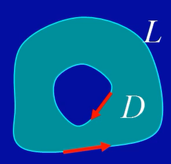
区域D的分类
单连通区域(无洞区域)
多连通区域(有洞区域)
域D边界L的正向:域的内部靠左,这两个方向都是正向
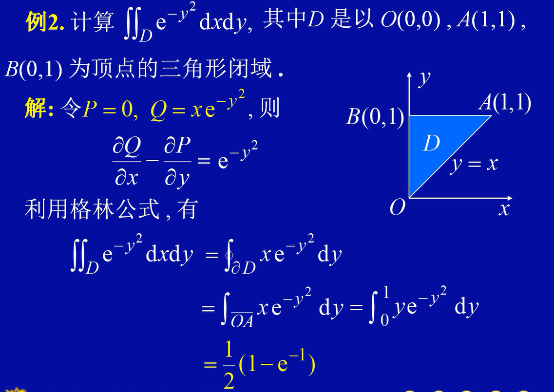
设区域D是由分段光滑正向曲线L围成,函数P(x,y),Q(x,y)在D上具有连续的一阶偏导数。则有
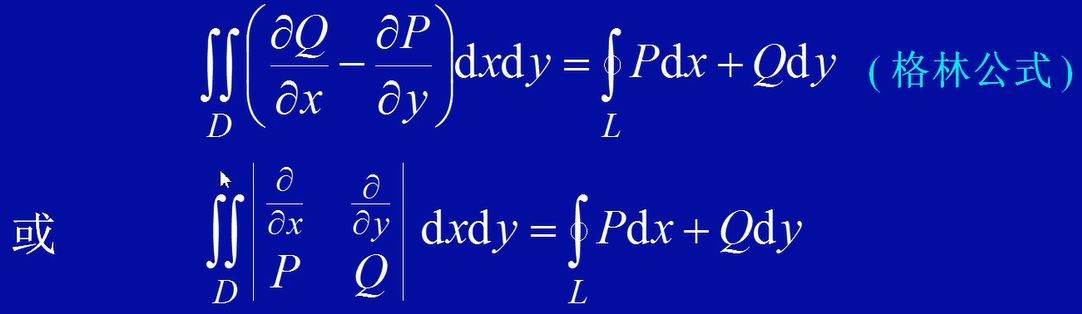
根据格林公式:正向闭曲线L所围成的区域D的面积
注意,格林公式的P跟dx,所以上面的P是-y,Q是x
椭圆
所围成的面积
正向格林公式
逆向格林公式:
这道题目,需要用逆向思维,把现在的函数倒退成未进行格林公式变形时的积分。然后还需要转几个弯。利用坐标的曲线积分求解的时候,需要判断出
都为0,只需要求即可
分类讨论:
设D 是单连通区域,函数P(x,y),Q(x,y)在D内具有异界连续偏导数,则下列四个条件等价
根据定理,若某区域D内