原文链接:

Understanding how LLM inference works with llama.cpp

在这篇文章中，我们将深入探讨大语言模型（LLMs）的内部原理，以便在实践中了解它们是如何工作的。为了帮助我们进行这项探索，我们将使用llama.cpp的源代码，这是Meta的LLaMA模型的纯C++实现。就我个人而言，我发现llama.cpp对于深入理解LLMs非常有帮助。它的代码简洁明了，没有过多的抽象。我们将使用这个提交版本进行讲解(https://github.com/ggerganov/llama.cpp/tree/7ddf185537b712ea0ccbc5f222ee92bed654914e)。

我们将关注LLMs的推理方面，也就是说：已经训练好的模型如何根据用户提示生成响应。

这篇文章是为那些非机器学习和人工智能领域的工程师撰写的，他们对更深入了解大语言模型感兴趣。文章从工程角度关注LLM的内部原理，而非从AI角度出发。因此，它并不需要具备丰富的数学或深度学习知识。

在这篇文章中，我们将从头到尾讲解推理过程，涵盖以下主题:

• 张量(Tensor): 简要概述如何使用张量进行数学运算，运算可能会卸载到GPU上
• 分词(Tokenization): 将用户的提示拆分为一个个词元或令牌(Token)的过程，LLM将其作为输入
• 嵌入(Embedding): 将词元转换为向量表示的过程
• Transformer：LLM架构的核心部分，负责实际的推理过程。我们将关注自注意力机制
• 采样(Sampling)：选择下一个预测词元的过程。我们将探讨两种采样技术
• KV缓存：用于加速大型提示中推理的常用优化技术。我们将探讨一个基本的kv缓存实现

从输入提示到输出的整体流程

作为一个大语言模型，LLaMA通过接收提示（prompt），然后预测接下来的词元或单词进行工作。

为了说明这一点，我们将使用关于量子力学的维基百科文章的第一句作为例子。我们的提示是：

LLM试图根据其训练所得到的最可能的词元来继续这个句子。使用llama.cpp，我们得到：

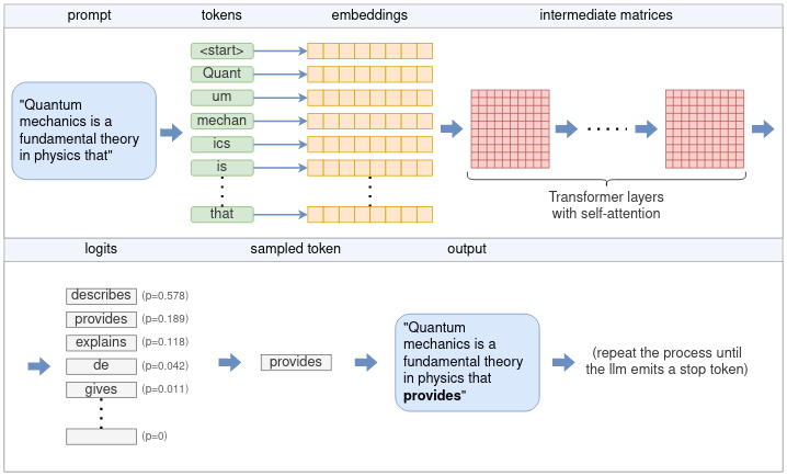
我们从研究这个过程的整体流程开始。从核心来看，LLM每次只预测一个词元。通过反复将LLM模型应用于相同的提示，并将之前的输出词元附加到提示上，实现生成完整句子（或更多）。这种类型的模型被称为自回归模型。因此，我们的关注点主要是生成单个标记，如下示意图所示：
(从用户提示生成单个词元的完整流程包括多个阶段，例如分词、嵌入、Transformer神经网络和采样)

上图的流程描述如下：

1. 分词器将提示分割成一个词元列表。根据模型的词汇表，某些单词可能会被拆分成多个词元。每个词元由一个唯一的数字表示；
2. 每个数值标记都会转换成一个嵌入。嵌入是一个固定大小的向量，这种方式来表征词元便于LLM处理。所有的嵌入一起形成一个嵌入矩阵；
3. 嵌入矩阵作为输入送入Transformer。Transformer是一个神经网络，是LLM的核心。Transformer由多个层组成的链条构成。每层接收一个输入矩阵，并使用模型参数对其进行各种数学运算，最显著的是自注意力机制。该层的输出被用作下一层的输入；
4. 一个最终的神经网络将Transformer的输出转换成logits。每个可能的下一个词元都有一个对应的logits，表示该词元是句子的“正确”延续的概率；
5. 从logits列表中选择下一个词元时，会使用某种抽样技术从列表中选取一个使用；
6. 选择的词元作为输出返回。要继续生成词元，则将所选词元附加到步骤1中的词元列表中，并重复该过程，直到生成所需数量的词元，或者LLM发出一个特殊的结束流（EOS）标记。

在接下来的部分中，我们将深入探讨各个步骤。在此之前，我们先需要熟悉基本的数据结构张量。

理解使用ggml的张量

张量是在神经网络中执行数学运算的主要数据结构。llama.cpp 使用 ggml，这是一个纯 C++ 的张量实现，相当于 Python 生态系统中的 PyTorch 或 TensorFlow。我们将使用 ggml 来了解张量的操作方式。

张量表示一个多维数组的数字。张量可以容纳一个单独的数字、一个向量（一维数组）、一个矩阵（二维数组）,甚至三维或四维数组。实际应用中，不需要更多维度。

区分两种类型的张量非常重要。有一种张量包含实际数据，它们包含一个多维数字数组。另一方面，有些张量只表示一个或多个其他张量之间计算的结果，并且在实际计算之前不包含数据。下文会探讨这种区别。

张量的基本结构

在ggml中，张量由ggml_tensor结构表示。为了简化说明，它的结构如下：

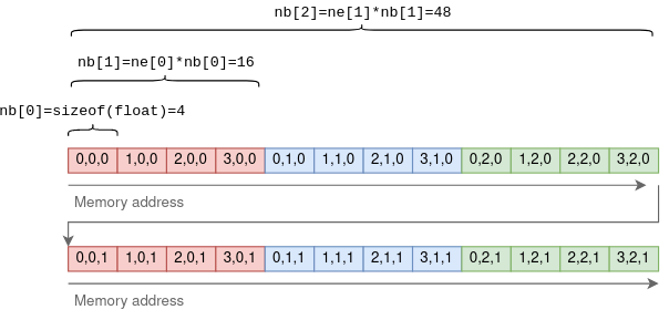
• type字段包含张量元素的原始类型。例如，GGML_TYPE_F32表示每个元素都是一个32位浮点数。
• enum字段表示张量是由CPU支持还是GPU支持。
• n_dims表示张量的维度数量，其范围可以从1到4。
• ne表示每个维度中的元素数量。GGML采用行优先顺序，这意味着ne[0]表示每行的大小，ne[1]表示每列的大小，以此类推。
• nb稍微复杂一些。它包含了步长（stride）：不同维度相邻元素之间的字节数。在第一个维度中，这将是原始元素的大小。在第二个维度中，它将是行大小乘以元素的大小，以此类推。以一个4x3x2的张量为例：
  使用步长的目的是允许执行某些张量操作而无需复制任何数据。例如，在一个二维张量上执行转置操作，将行变为列，可以通过仅交换ne和nb并指向相同的底层数据来完成：

在上述函数中，result是一个新的张量，初始化为指向与源张量a相同的多维数字数组。通过交换ne中的维度和nb中的步幅，它在不复制任何数据的情况下执行转置操作。

张量操作和视图

正如之前提到的，一些张量包含数据，而其他张量表示其他张量之间操作的理论结果。回到struct ggml_tensor：

• op 可以是支持的张量之间的任意操作。将其设置为 GGML_OP_NONE 表示张量包含数据。其他值可以表示一种操作。例如，GGML_OP_MUL_MAT 表示这个张量不包含数据，而仅仅表示两个其他张量之间的矩阵乘法结果。
• src 是一个指针数组，用于存储进行操作的张量的指针。例如，如果 op == GGML_OP_MUL_MAT，那么 src 将包含两个待相乘张量的指针。如果 op == GGML_OP_NONE，那么 src 将为空。
• data 指向实际张量的数据，如果这个张量是一个操作，则为 NULL。它还可以指向另一个张量的数据，这时它被称为视图（view）。例如，在上面的 ggml_transpose() 函数中，结果张量是原始张量的一个视图，只是维度和步幅翻转了。data 指向内存中的相同位置。

矩阵乘法函数很好地展示了这些概念：

在上述函数中，result 不包含任何数据。它仅仅是乘以 a 乘 b 的理论结果的一个表示。

计算张量

上面的 ggml_mul_mat() 函数或任何其他张量操作，并不进行任何计算，而仅仅是为操作准备张量。从另一个角度来看，它构建了一个计算图，其中每个张量操作是一个节点，操作的源是节点的子节点。在矩阵乘法场景中，图有一个带有 GGML_OP_MUL_MAT 操作的父节点，以及两个子节点。

以下代码实现了自注意力机制，这是每个 Transformer 层的一部分，稍后将对其进行更深入的探讨：

该代码是一系列张量操作，并构建了一个与原始 Transformer 论文中描述的相同的计算图：

为了计算结果张量（这里是 KQV）的实际值，需要执行以下步骤：

1. 将数据加载到每个叶子张量的数据指针中。在这个例子中，叶子张量是 K、Q 和 V。
2. 使用 ggml_build_forward() 函数将输出张量（KQV）转换为计算图。这个函数相对简单，以深度优先顺序对节点进行排序。
3. 通过使用 ggml_graph_compute() 函数运行计算图，它以深度优先顺序对每个节点运行 ggml_compute_forward()。ggml_compute_forward() 负责执行复杂数学计算。它执行数学运算并将结果填充到张量的数据指针中。
4. 在这个过程的最后，输出张量的数据指针指向最终结果。

将计算卸载到 GPU

许多张量操作，如矩阵加法和乘法，由于 GPU 的高并行性，可以在 GPU 上进行更高效的计算。当 GPU 可用时，可以使用 tensor->backend = GGML_BACKEND_GPU 标记张量。在这种情况下，ggml_compute_forward() 将尝试将计算卸载到 GPU。GPU 将执行张量操作，并将结果存储在 GPU 的内存中（而不是数据指针中）。

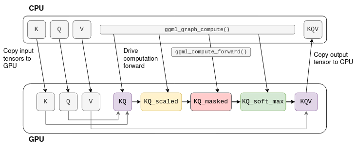
考虑之前展示的自注意力计算图。假设 K、Q、V 是固定的张量，那么计算可以卸载到 GPU：

该过程首先将 K、Q、V 复制到 GPU 内存中。然后，CPU 逐张量地驱动GPU计算，实际的数学运算被卸载到 GPU 上。当计算图中的最后一个操作结束时，结果张量的数据将从 GPU 内存复制回 CPU 内存。

注： 在实际的 Transformer 中，K、Q、V 并非固定的，而且 KQV 并非最终输出。稍后将进一步讨论这个问题。

分词

推理的第一步是分词。分词是将输入文本分割成一个个较短字符串（称为词元）的过程。这些词元必须是模型词汇表中的一部分，词汇表包含了大型语言模型在训练过程中用到的词元。例如，LLaMA 的词汇表包含 32k 个词元，并作为模型的一部分分发。

对于我们的示例输入，分词将其拆分为十一个令牌（空格被替换为特殊的元符号 ‘▁’（U+2581））：

在分词过程中，LLaMA 使用了 SentencePiece 分词器和字节对编码（BPE）算法。这个分词器之所以引人关注，是因为它基于子词，这意味着一个单词可能由多个令牌表示。例如，在我们的输入文本中，“Quantum”被拆分为“Quant”和“um”。在训练过程中，当词汇表被构建时，BPE 算法确保常见单词作为一个单独的令牌被包含在词汇表中，而罕见单词(出现频率低)被拆分为子词。在上面的示例中，单词“Quantum”不包含在词汇表中，但“Quant”和“um”作为两个单独的令牌包含在内。空格没有被特殊对待，如果它们足够常见，它们会被包含在令牌本身中，作为元字符。

基于子词的分词方法之所以强大，有以下几个原因：

• 基于子词的分词方法使得大型语言模型（LLM）在保持词汇表相对较小的同时，通过将常见的后缀和前缀表示为单独的令牌，学习诸如“Quantum”之类罕见词汇的含义。
• 它学习特定于语言的特征，而无需使用特定于语言的分词方案。
• 同样，在解析代码时也很有用。例如，一个名为 model_size 的变量将被标记化为 model|_|size，这使得 LLM 能够“理解”变量的用途。

在 llama.cpp 中，使用 llama_tokenize() 函数执行分词。该函数将提示字符串作为输入，并返回一个由整数表示的标记列表，其中每个标记都由一个整数表示：

分词过程首先将输入分解为单词元（即单个字符），迭代地尝试将每两个连续的词元合并为一个更大的词元，只要合并后的词元是词汇表的一部分。这确保了生成的词元尽可能大。对于我们的示例输入，分词步骤如下：

请注意，每个中间步骤都根据模型的词汇表进行有效的标记化。然而，只有最后一个被用作 LLM（大型语言模型）的输入。

嵌入

这些词元被用作输入到LLaMA，以预测下一个词元。这里的关键函数是 llm_build_llama() 函数：

这个函数以tokens和n_tokens参数表示的词元列表作为输入。然后，它构建LLaMA的完整张量计算图，并将其作为一个名为ggml_cgraph的结构体返回。在这个阶段，实际上并没有进行任何计算。n_past参数当前被设置为零，现在可以先忽略它。在讨论kv缓存时，会介绍它的作用。

除了词元之外，该函数还使用了模型权重或模型参数。这些是在LLM训练过程中学习到的固定张量，并且是模型的一部分。在推理开始之前，这些模型参数会被预先加载到lctx中。

现在我们开始探索计算图的结构。计算图的第一部分涉及将令牌转换为嵌入向量。

嵌入向量是每个词元的固定向量表示，它比纯整数更适合深度学习，因为它捕获了单词的语义含义。这个向量的大小是模型维度，不同的模型这个维度会有所不同。例如，在LLaMA-7B中，模型维度n_embd为4096。

模型参数中包括一个词元嵌入矩阵，它负责将令牌转换为嵌入向量。由于我们的词汇量大小n_vocab为32000，所以这是一个32000 x 4096的矩阵，其中每一行都包含一个令牌的嵌入向量。

(每个令牌都有一个与之关联的嵌入向量，这个嵌入向量是在训练过程中学习得到的，并且作为令牌嵌入矩阵的一部分可供访问。)

计算图的第一部分是从令牌嵌入矩阵中提取每个令牌对应的相关行：

代码首先创建一个新的一维整数张量，称为inp_tokens，用于存储数值令牌。然后，它将令牌值复制到该张量的数据指针中。最后，它创建一个新的GGML_OP_GET_ROWS张量操作，该操作将令牌嵌入矩阵model.tok_embeddings与我们的令牌结合起来。

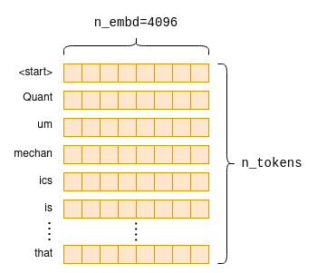
这个操作在稍后进行计算时，会按照上述图表的方式从嵌入矩阵中提取行，从而创建一个新的n_tokens x n_embd矩阵，该矩阵仅包含按原始顺序排列的令牌嵌入向量:

Transformer

计算图的主要部分被称为Transformer。Transformer是一种神经网络架构，它是LLM的核心，并执行主要的推理逻辑。在接下来的部分，我们将从工程角度探索Transformer的一些关键方面，重点关注自注意力机制。如果你想要了解Transformer架构背后的原理，参考阅读《图解Transformer》。

self-attention(自注意力)

我们首先深入了解自注意力是什么；之后，我们将回到整体，看看它如何融入Transformer架构中。

自注意力是一种机制，它接受一系列令牌，并生成这个序列的紧凑向量表示，同时考虑到令牌之间的关系。在LLM架构中，这是唯一计算令牌之间关系的地方。因此，它构成了语言理解的核心，语言理解包括理解单词之间的关系。由于它涉及跨令牌的计算，从工程角度来看，它也是最有趣的地方，因为计算量可能会变得相当大，尤其是对于较长的序列。

自注意力机制的输入是n_tokens x n_embd嵌入矩阵，其中每一行或向量代表一个单独的令牌。然后，这些向量中的每一个都被转换为三个不同的向量，称为“key”、“query”和“value”向量。这种转换是通过将每个令牌的嵌入向量与固定矩阵wk、wq和wv相乘来实现的，这些矩阵是模型参数的一部分：

这个过程对于每个令牌都是重复的，即进行n_tokens次。理论上，这可以在一个循环中完成，但为了效率，所有行都通过矩阵乘法在单个操作中完成转换，这正是矩阵乘法所做的。相关代码看起来如下：

最终，我们得到了K、Q和V这三个矩阵，它们的尺寸也都是n_tokens x n_embd，分别包含了每个令牌的键向量、查询向量和值向量。

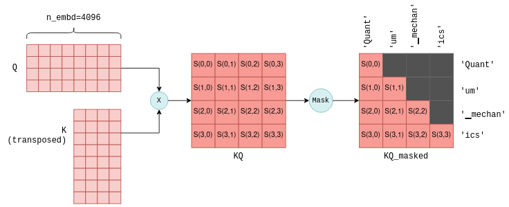
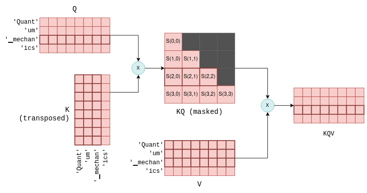
自注意力机制的下一步是将包含堆叠查询向量的矩阵Q与包含堆叠键向量的矩阵K的转置相乘。对于不太熟悉矩阵运算的人来说，这个操作基本上是为每一对查询和键向量计算一个联合得分。我们将使用S(i,j)的符号来表示查询i与键j的得分。

这个过程会产生n_tokens^2个得分，每个查询-键对都有一个，它们被打包在一个称为KQ的单一矩阵中。随后，这个矩阵会被遮罩以去除对角线上方的条目：

(通过将Q与K的转置相乘，为每个查询-键对计算一个联合得分S(i,j)。这里展示的结果是前四个令牌的得分，以及每个得分所代表的令牌。遮罩步骤确保只保留一个令牌与其之前令牌之间的得分。为了简化，这里省略了中间的缩放操作。)

遮罩操作是一个关键步骤。对于每个令牌，它只保留与其之前令牌的得分。在训练阶段，这一约束确保LLM（大型语言模型）学会仅根据过去的令牌来预测令牌，而不是未来的令牌。此外，正如我们稍后将更详细地探讨的，这在预测未来令牌时允许进行显著的优化。

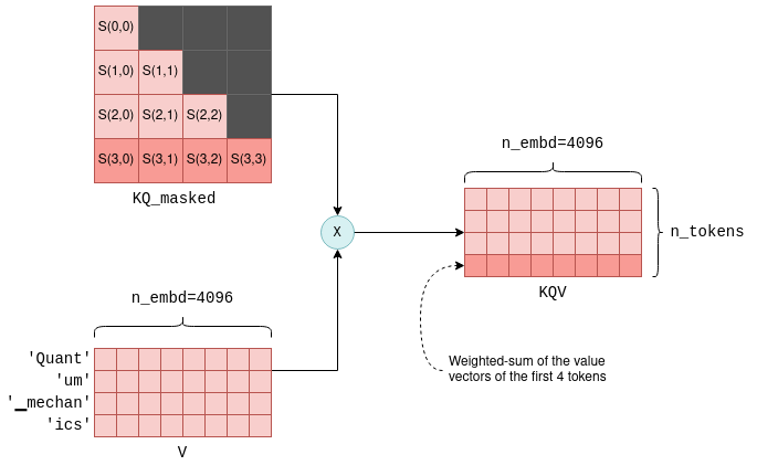
自注意力机制的最后一步是将遮罩后的得分KQ_masked与之前的值向量相乘。这样的矩阵乘法操作会创建所有之前令牌值向量的加权和，其中权重是得分S(i,j)。例如，对于第四个令牌“ics”，它会根据权重S(3,0)到S(3,3)来创建“Quant”、“um”、“mechan”和“ics”值向量的加权和，这些权重自身是根据“ics”的查询向量和所有之前键向量计算得出的。

(KQV矩阵包含值向量的加权和。例如，高亮显示的最后一行是前四个值向量的加权和，权重是高亮显示的得分。)

KQV矩阵完成了自注意力机制。实现自注意力机制的相关代码之前已经在一般张量计算的上下文中呈现过了，但现在你更充分地理解了它。

Transformer的层

自注意力是被称为Transformer层中的组件之一。每一层除了自注意力机制外，还包含多个其他的张量操作，主要是前馈神经网络中的矩阵加法、乘法和激活函数。我们不会深入探讨这些内容的细节，但只需注意以下事实：

• 在前馈网络中使用了大型、固定的参数矩阵。在LLaMA-7B中，它们的大小是n_embd x n_ff = 4096 x 11008。
• 除了自注意力之外，所有其他操作都可以认为是逐行或逐令牌进行的。如前所述，只有自注意力包含跨令牌的计算。这在稍后讨论kv-cache时将变得非常重要。
• 输入和输出的尺寸始终是n_tokens x n_embd：每个令牌一行，每行的尺寸与模型的维度相同。

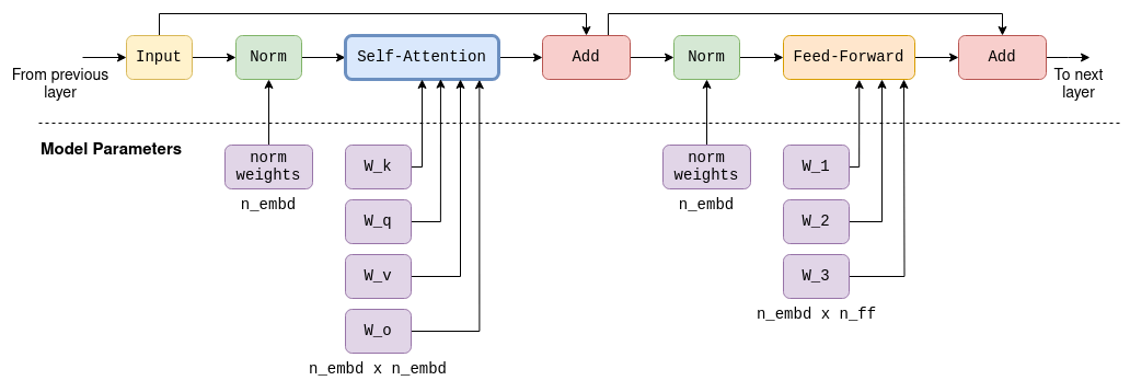
为了完整性，我包含了LLaMA-7B中一个Transformer层的示意图。请注意，未来的模型确切架构很可能会略有不同：

(LLaMA-7B中Transformer层的完整计算图，包含自注意力机制和前馈机制。每一层的输出都作为下一层的输入。在自注意力阶段和前馈阶段都使用了大型参数矩阵。这些构成了模型70亿参数中的大部分。)

在Transformer架构中，有多个层。例如，在LLaMA-7B中，有n_layers=32层。这些层是相同的，只是每一层都有自己的一套参数矩阵（例如，用于自注意力机制的wk、wq和wv矩阵）。第一层的输入是上述的嵌入矩阵。第一层的输出然后用作第二层的输入，以此类推。我们可以将其视为每一层都生成一个嵌入列表，但每个嵌入不再直接绑定到单个令牌，而是绑定到对令牌关系的某种更复杂理解上。

计算logits

Transformer的最后一步涉及logits的计算。Logit是一个浮点数，表示特定令牌是“正确”的下一个令牌的概率。Logit的值越高，对应的令牌是“正确”令牌的可能性就越大。

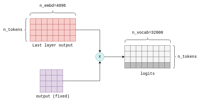
logits是通过将Transformer最后一层的输出与一个固定的n_embd x n_vocab参数矩阵（在llama.cpp中也称为output）相乘来计算的。这个操作会为词汇表中的每个令牌生成一个logit。例如，在LLaMA中，它会生成n_vocab=32000个logits：

(Transformer的最后一步是通过将最后一层的输出与一个固定的参数矩阵（也称为“输出”）相乘来计算logits的。只有结果中的最后一行（在此处高亮显示）是关注的重点，它包含了词汇表中每个可能下一个令牌的logit。)

logits是Transformer的输出，它告诉我们最可能的下一个令牌是什么。至此，所有的张量计算都已完成。以下是一个简化并带有注释的llm_build_llama()函数版本，它概括了本节中描述的所有步骤：

为了实际执行推理，会使用之前描述的ggml_graph_compute()函数来计算这个函数返回的计算图。然后，将logits从最后一个张量的数据指针中复制到一个浮点数数组中，为下一步的采样操作做好准备。

sampling

在获得logits列表后，下一步是基于这些logits来选择下一个令牌。这个过程被称为采样。有多种采样方法可供选择，适用于不同的用例。在本节中，我们将介绍两种基本的采样方法，而将更高级的采样方法（如语法采样）留待后续文章介绍。

Greedy Sampling(贪婪采样)

贪婪采样是一种直接的方法，它选择与其关联的logits值最高的令牌。

以我们的示例提示为例，以下令牌具有最高的logits值：

token	logit
▁describes	18.990
▁provides	17.871
▁explains	17.403
▁de	16.361
▁gives	15.007
因此，贪婪采样将确定性地选择“describes”作为下一个令牌。当重新评估相同提示时需要确定性输出时，贪婪采样最有用。

Temperature sampling(温度采样)

温度采样是概率性的，这意味着相同的提示在重新评估时可能会产生不同的输出。它使用一个名为温度的参数，该参数是一个介于0和1之间的浮点数，会影响结果的随机性。这个过程如下：

1. logits从高到低进行排序，并使用softmax函数进行归一化，以确保它们的总和为1。这种转换将每个logit转换为概率。
2. 应用一个阈值（默认为0.95），仅保留顶部的令牌，使得它们的累积概率低于阈值。这一步有效地移除了低概率的令牌，防止“不好”或“不正确”的令牌被罕见地采样到。
3. 剩余的logits除以温度参数，并再次进行归一化，使得它们的总和为1并代表概率。
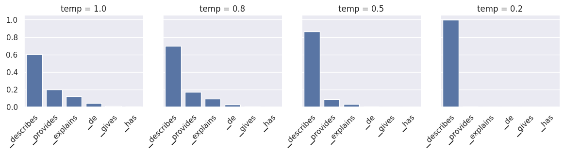
4. 基于这些概率随机采样一个令牌。例如，在我们的提示中，令牌“describes”具有概率p=0.6，这意味着它大约会被选择60%的时间。在重新评估时，可能会选择不同的令牌。

步骤3中的温度参数用于增加或减少随机性。较低的温度值会抑制低概率令牌，使得在重新评估时更有可能选择相同的令牌。因此，较低的温度值会降低随机性。相反，较高的温度值往往会“平滑”概率分布，强调低概率令牌。这增加了每次重新评估产生不同令牌的可能性，从而增加了随机性。

(对于我们示例提示的下一个令牌概率进行归一化。较低的温度会抑制低概率令牌，而较高的温度会强调它们。temp=0基本上与贪婪采样相同。)

采样一个令牌标志着大型语言模型（LLM）的一次完整迭代结束。在令牌被采样后，它被添加到令牌列表中，然后整个过程再次运行。输出迭代地成为LLM的输入，每次迭代增加一个令牌。

理论上，后续的迭代可以完全相同地进行。然而，为了解决随着令牌列表增长而出现的性能下降问题，采用了某些优化方法。这些将在接下来进行介绍。

优化推理

随着输入到大语言模型（LLM）的令牌列表的增长，Transformer的自注意力阶段可能成为性能瓶颈。更长的令牌列表意味着更大的矩阵需要相乘。每个矩阵乘法都包含许多较小的数值运算，即浮点运算，它们受到GPU每秒浮点运算次数（flops）能力的限制。在Transformer推理算术中，计算得出，对于520亿参数的模型，在A100 GPU上，由于过多的浮点运算，性能在208个令牌时开始下降。解决这一瓶颈最常用的优化技术被称为kv缓存。

KV Cache

总结来说，每个令牌都与一个嵌入向量相关联，该嵌入向量通过与参数矩阵wk和wv相乘，进一步转换为键向量和值向量。kv缓存就是这些键向量和值向量的缓存。通过缓存它们，我们节省了每次迭代时重新计算它们所需的浮点运算。

缓存的工作原理如下：

• 在初始迭代中，根据之前描述的方法，为所有令牌计算键向量和值向量，然后将其保存到kv缓存中。
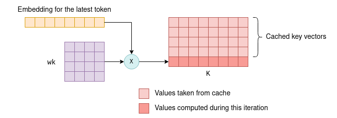
• 在后续的迭代中，只需要计算最新令牌的键向量和值向量。将缓存的k-v向量与新令牌的k-v向量拼接在一起，形成K和V矩阵。这节省了重新计算所有先前令牌的k-v向量的时间，这在性能上是非常重要的。
  

(在后续的迭代中，仅计算最新令牌的键向量。其余键向量从缓存中提取，它们共同组成K矩阵。新计算出的键向量也会被保存到缓存中。对值向量的处理也遵循相同的过程。)

能够利用缓存来存储键向量和值向量，是因为这些向量在迭代之间保持不变。例如，如果我们首先处理四个令牌，然后再处理五个令牌（其中前四个令牌保持不变），那么在第一次和第二次迭代之间，前四个键向量和值向量将保持不变。因此，在第二次迭代中，无需重新计算前四个令牌的键向量和值向量。

这个原理不仅适用于Transformer的第一层，也适用于其所有层。在所有层中，每个令牌的键向量和值向量仅依赖于之前的令牌。因此，随着后续迭代中不断添加新令牌，现有令牌的键向量和值向量保持不变。

对于第一层来说，这个概念相对容易验证：令牌的键向量是通过将令牌的固定嵌入与固定的wk参数矩阵相乘来确定的。因此，无论引入了多少额外的令牌，在后续的迭代中，它都保持不变。同样的逻辑也适用于值向量。

对于第二层及之后的层，这个原理可能不太明显，但仍然成立。为了理解这一点，请考虑第一层输出的KQV矩阵，即自注意力阶段的输出。KQV矩阵中的每一行都是一个加权和，它依赖于：

• 之前令牌的值向量
• 根据之前令牌的键向量计算出的得分

因此，KQV矩阵中的每一行仅依赖于之前的令牌。这个矩阵在经过一些额外的基于行的操作后，将作为第二层的输入。这意味着在后续的迭代中，除了新添加的行之外，第二层的输入将保持不变。通过归纳，相同的逻辑可以扩展到其余层。

(再来看一下KQV矩阵是如何计算的。高亮显示的第三行仅基于第三个查询向量和前三个键向量和值向量（也已高亮）来确定。后续的令牌不会影响它。因此，在未来的迭代中，它将保持不变。)

进一步优化后续迭代

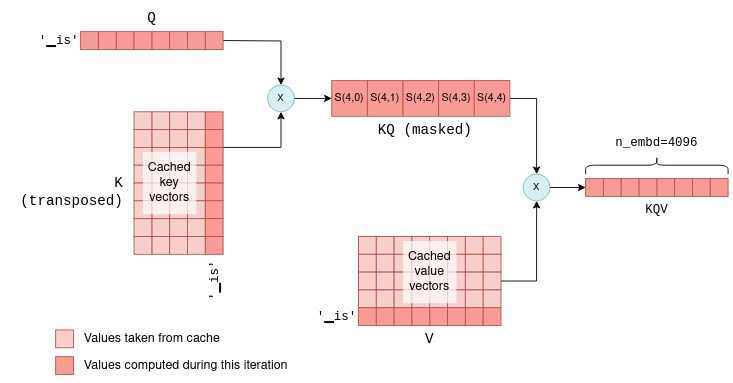
既然我们缓存了键向量和值向量，为什么不缓存查询向量？答案是，除了当前令牌的查询向量之外，在后续迭代中，我们其实并不需要之前令牌的查询向量。有了kv缓存，我们实际上只需要将最新的令牌的查询向量输入到自注意力机制中。这个查询向量会与缓存的K矩阵相乘，以计算最后一个令牌与所有之前令牌之间的联合得分。然后，它再与缓存的V矩阵相乘，以仅计算KQV矩阵的最新一行。事实上，在所有层中，我们现在传递的是大小为1 x n_embd的向量，而不是在第一次迭代中计算得到的n_token x n_embd大小的矩阵。为了说明这一点，请比较以下图表，它显示了后续的迭代，与之前的图表相比：

(后续迭代中的自注意力机制。在这个例子中，第一次迭代中有四个令牌，而第二次迭代中添加了一个第五个令牌“is”。最新的令牌的键向量、查询向量和值向量，与缓存的键向量和值向量一起，用于计算KQV矩阵的最后一行，而这正是预测下一个令牌所需的全部内容。)

这个过程在所有层中重复进行，利用每一层的KV缓存。因此，在这种情况下Transformer的输出是一个单独的长度为n_vocab的logits向量，用于预测下一个令牌。

通过这种优化，我们节省了计算 KQ 和 KQV 中不必要行的浮点运算，这在标记列表的大小增长时可能会变得非常显著。

KV缓存的实战运用

我们可以深入探究 llama.cpp 代码，以了解 kv 缓存在实际中是如何实现的。也许这并不令人意外，kv 缓存是通过使用张量来构建的，一个用于存储键向量，另一个用于存储值向量：

当缓存被初始化时，会分配足够的空间来存储每一层的 512 个键向量和值向量：

回想一下，在推理过程中，计算图是通过函数 llm_build_llama() 来构建的。这个函数有一个之前我们忽略的参数，叫做 n_past。在第一次迭代中，n_tokens 参数包含标记的数量，而 n_past 被设置为 0。在后续的迭代中，n_tokens 被设置为 1，因为只处理最新的标记，而 n_past 包含过去标记的数量。然后，n_past 用于从 kv 缓存中拉取正确数量的键和值向量。

这个函数中相关的部分如下所示，它利用缓存来计算 K 矩阵。为了简化，我忽略了多头注意力，并为每个步骤添加了注释：

首先，计算新的键向量。然后，使用 n_past 来查找缓存中的下一个空槽，并将新的键向量复制到这里。最后，通过获取缓存中具有正确标记数量（n_past + n_tokens）的视图来形成矩阵 K。

kv 缓存是 LLM 推理优化的基础。值得注意的是，在 llama.cpp 中实现（截至本文写作时）并在此处呈现的版本并不是最优的版本。例如，它预先分配了大量内存来存储支持的最大键和值向量数量（在此为 512）。更高级的实现，如 vLLM，旨在提高内存使用效率，并可能提供进一步的性能提升。这些高级技术将留待未来的文章介绍。此外，随着这个领域的飞速发展，未来可能会出现新的和改进的优化技术。

总结

这篇文章涵盖了很多内容，应该能让你对 LLM 推理的全过程有一个基本的了解。有了这些知识，你就可以更深入地了解更高级的资源：

• LLM 参数计数(LLM Parameter counting)和 Transformer 推理算术(Transformer Inference Arithmetic)深入分析了 LLM 的性能。
• vLLM 是一个用于更有效地管理 kv 缓存内存的库。
• 连续批处理是一种优化技术，用于将多个 LLM 提示组合在一起进行批处理。

附注

1. ggml 还提供了 ggml_build_backward() 函数，该函数从输出到输入以反向方式计算梯度。这仅在模型训练期间用于反向传播，而在推理过程中从未使用。
2. 本文描述了一个编码器-解码器模型。然而，LLaMA 是一个仅解码器模型，因为它一次只预测一个标记。但核心概念是相同的。
3. 为了简化说明，我选择了在这里描述单头自注意力机制。然而，LLaMA 使用的是多头自注意力机制。除了使张量操作稍微复杂一些外，它对本节介绍的核心思想没有任何影响。
4. 准确地说，嵌入向量首先会经过一个标准化操作，对其值进行缩放。我们忽略了这一点，因为它并不影响所介绍的核心思想。
5. 得分也经过一个 softmax 操作，该操作对其进行缩放，使得每行得分的总和为 1。

In this post, we will dive into the internals of Large Language Models (LLMs) to gain a practical understanding of how they work. To aid us in this exploration, we will be using the source code of llama.cpp, a pure c++ implementation of Meta’s LLaMA model.Personally, I have found llama.cpp to be an excellent learning aid for understanding LLMs on a deeper level. Its code is clean, concise and straightforward, without involving excessive abstractions.We will use this commit version.

We will focus on the inference aspect of LLMs, meaning: how the already-trained model generates responses based on user prompts.

This post is written for engineers in fields other than ML and AI who are interested in better understanding LLMs.It focuses on the internals of an LLM from an engineering perspective, rather than an AI perspective.Therefore, it does not assume extensive knowledge in math or deep learning.

Throughout this post, we will go over the inference process from beginning to end, covering the following subjects (click to jump to the relevant section):

• Tensors: A basic overview of how the mathematical operations are carried out using tensors, potentially offloaded to a GPU.
• Tokenization: The process of splitting the user’s prompt into a list of tokens, which the LLM uses as its input.
• Embedding: The process of converting the tokens into a vector representation.
• The Transformer: The central part of the LLM architecture, responsible for the actual inference process. We will focus on the self-attention mechanism.
• Sampling: The process of choosing the next predicted token. We will explore two sampling techniques.
• The KV cache: A common optimization technique used to speed up inference in large prompts. We will explore a basic kv cache implementation.

By the end of this post you will hopefully gain an end-to-end understanding of how LLMs work. This will enable you to explore more advanced topics, some of which are detailed in the last section.

Table of contents

High-level flow from prompt to output

As a large language model, LLaMA works by taking an input text, the “prompt”, and predicting what the next tokens, or words, should be.

To illustrate this, we will use the first sentence from the Wikipedia article about Quantum Mechanics as an example.Our prompt is:

Quantum mechanics is a fundamental theory in physics that

The LLM attempts to continue the sentence according to what it was trained to believe is the most likely continuation.Using llama.cpp, we get the following continuation:

provides insights into how matter and energy behave at the atomic scale.

Let’s begin by examining the high-level flow of how this process works.At its core, an LLM only predicts a single token each time.The generation of a complete sentence (or more) is achieved by repeatedly applying the LLM model to the same prompt, with the previous output tokens appended to the prompt.This type of model is referred to as an autoregressive model.Thus, our focus will primarily be on the generation of a single token, as depicted in the high-level diagram below:

Following the diagram, the flow is as follows:

1. The tokenizer splits the prompt into a list of tokens. Some words may be split into multiple tokens, based on the model’s vocabulary. Each token is represented by a unique number.
2. Each numerical token is converted into an embedding. An embedding is a vector of fixed size that represents the token in a way that is more efficient for the LLM to process. All the embeddings together form an embedding matrix.
3. The embedding matrix serves as the input to the Transformer. The Transformer is a neural network that acts as the core of the LLM. The Transformer consists of a chain of multiple layers. Each layer takes an input matrix and performs various mathematical operations on it using the model parameters, the most notable being the self-attention mechanism. The layer’s output is used as the next layer’s input.
4. A final neural network converts the output of the Transformer into logits. Each possible next token has a corresponding logit, which represents the probability that the token is the “correct” continuation of the sentence.
5. One of several sampling techniques is used to choose the next token from the list of logits.
6. The chosen token is returned as the output. To continue generating tokens, the chosen token is appended to the list of tokens from step (1), and the process is repeated. This can be continued until the desired number of tokens is generated, or the LLM emits a special end-of-stream (EOS) token.

In the following sections, we will delve into each of these steps in detail.But before doing that, we need to familiarize ourselves with tensors.

Understanding tensors with ggml

Tensors are the main data structure used for performing mathemetical operations in neural networks.llama.cpp uses ggml, a pure C++ implementation of tensors, equivalent to PyTorch or Tensorflow in the Python ecosystem.We will use ggml to get an understanding of how tensors operate.

A tensor represents a multi-dimensional array of numbers. A tensor may hold a single number, a vector (one-dimensional array), a matrix (two-dimensional array) or even three or four dimensional arrays. More than is not needed in practice.

It is important to distinguish between two types of tensors.There are tensors that hold actual data, containing a multi-dimensional array of numbers.On the other hand, there are tensors that only represent the result of a computation between one or more other tensors, and do not hold data until actually computed.We will explore this distinction soon.

Basic structure of a tensor

In ggml tensors are represented by the ggml_tensor struct. Simplified slightly for our purposes, it looks like the following:

// ggml.hstruct ggml_tensor {    enum ggml_type    type;    enum ggml_backend backend;    int     n_dims;    // number of elements    int64_t ne[GGML_MAX_DIMS];    // stride in bytes    size_t  nb[GGML_MAX_DIMS];    enum ggml_op op;    struct ggml_tensor * src[GGML_MAX_SRC];    void * data;    char name[GGML_MAX_NAME];};

The first few fields are straightforward:

• type contains the primitive type of the tensor’s elements. For example, GGML_TYPE_F32 means that each element is a 32-bit floating point number.
• enum contains whether the tensor is CPU-backed or GPU-backed. We’ll come back to this bit later.
• n_dims is the number of dimensions, which may range from 1 to 4.
• ne contains the number of elements in each dimension. ggml is row-major order, meaning that ne[0] marks the size of each row, ne[1] of each column and so on.

nb is a bit more sophisticated. It contains the stride: the number of bytes between consequetive elements in each dimension. In the first dimension this will be the size of the primitive element. In the second dimension it will be the row size times the size of an element, and so on. For example, for a 4x3x2 tensor:

The purpose of using a stride is to allow certain tensor operations to be performed without copying any data.For example, the transpose operation on a two-dimensional that turns rows into columns can be carried out by just flipping ne and nb and pointing to the same underlying data:

// ggml.c (the function was slightly simplified).struct ggml_tensor * ggml_transpose(        struct ggml_context * ctx,        struct ggml_tensor  * a) {    // Initialize `result` to point to the same data as `a`    struct ggml_tensor * result = ggml_view_tensor(ctx, a);    result->ne[0] = a->ne[1];    result->ne[1] = a->ne[0];    result->nb[0] = a->nb[1];    result->nb[1] = a->nb[0];    result->op   = GGML_OP_TRANSPOSE;    result->src[0] = a;    return result;}

In the above function, result is a new tensor initialized to point to the same multi-dimensional array of numbers as the source tensor a.By exchanging the dimensions in ne and the strides in nb, it performs the transpose operation without copying any data.

Tensor operations and views

As mentioned before, some tensors hold data, while others represent the theoretical result of an operation between other tensors.Going back to struct ggml_tensor:

• op may be any supported operation between tensors. Setting it to GGML_OP_NONE marks that the tensor holds data. Other values can mark an operation. For example, GGML_OP_MUL_MAT means that this tensor does not hold data, but only represents the result of matrix multiplication between two other tensors.
• src is an array of pointers to the tensors between which the operation is to be taken. For example, if op == GGML_OP_MUL_MAT, then src will contain pointers to the two tensors to be multiplied. If op == GGML_OP_NONE, then src will be empty.
• data points to the actual tensor’s data, or NULL if this tensor is an operation. It may also point to another tensor’s data, and then it’s known as a view. For example, in the ggml_transpose() function above, the resulting tensor is a view of the original, just with flipped dimensions and strides. data points to the same location in memory.

The matrix multiplication function illustrates these concepts well:

// ggml.c (simplified and commented)struct ggml_tensor * ggml_mul_mat(        struct ggml_context * ctx,        struct ggml_tensor  * a,        struct ggml_tensor  * b) {    // Check that the tensors' dimensions permit matrix multiplication.    GGML_ASSERT(ggml_can_mul_mat(a, b));    // Set the new tensor's dimensions    // according to matrix multiplication rules.    const int64_t ne[4] = { a->ne[1], b->ne[1], b->ne[2], b->ne[3] };    // Allocate a new ggml_tensor.    // No data is actually allocated except the wrapper struct.    struct ggml_tensor * result = ggml_new_tensor(ctx, GGML_TYPE_F32, MAX(a->n_dims, b->n_dims), ne);    // Set the operation and sources.    result->op   = GGML_OP_MUL_MAT;    result->src[0] = a;    result->src[1] = b;    return result;}

In the above function, result does not contain any data. It is merely a representation of the theoretical result of multiplying a and b.

Computing tensors

The ggml_mul_mat() function above, or any other tensor operation, does not calculate anything but just prepares the tensors for the operation.A different way to look at it is that it builds up a computation graph where each tensor operation is a node, and the operation’s sources are the node’s children.In the matrix multiplication scenario, the graph has a parent node with operation GGML_OP_MUL_MAT, along with two children.

As a real example from llama.cpp, the following code implements the self-attention mechanism which is part of each Transformer layer and will be explored more in-depth later:

// llama.cppstatic struct ggml_cgraph * llm_build_llama(/* ... */) {    // ...    // K,Q,V are tensors initialized earlier    struct ggml_tensor * KQ = ggml_mul_mat(ctx0, K, Q);    // KQ_scale is a single-number tensor initialized earlier.    struct ggml_tensor * KQ_scaled = ggml_scale_inplace(ctx0, KQ, KQ_scale);    struct ggml_tensor * KQ_masked = ggml_diag_mask_inf_inplace(ctx0, KQ_scaled, n_past);    struct ggml_tensor * KQ_soft_max = ggml_soft_max_inplace(ctx0, KQ_masked);    struct ggml_tensor * KQV = ggml_mul_mat(ctx0, V, KQ_soft_max);    // ...}

The code is a series of tensor operations and builds a computation graph that is identical to the one described in the original Transformer paper: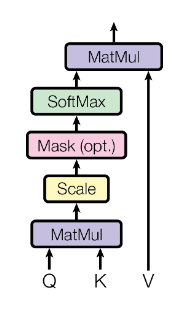

In order to actually compute the result tensor (here it’s KQV) the following steps are taken:

1. Data is loaded into each leaf tensor’s data pointer. In the example the leaf tensors are K, Q and V.
2. The output tensor (KQV) is converted to a computation graph using ggml_build_forward(). This function is relatively straightforward and orders the nodes in a depth-first order.¹
3. The computation graph is run using ggml_graph_compute(), which runs ggml_compute_forward() on each node in a depth-first order. ggml_compute_forward() does the heavy lifting of calculations. It performs the mathetmatical operation and fills the tensor’s data pointer with the result.
4. At the end of this process, the output tensor’s data pointer points to the final result.

Offloading calculations to the GPU

Many tensor operations like matrix addition and multiplication can be calculated on a GPU much more efficiently due to its high parallelism.When a GPU is available, tensors can be marked with tensor->backend = GGML_BACKEND_GPU.In this case, ggml_compute_forward() will attempt to offload the calculation to the GPU.The GPU will perform the tensor operation, and the result will be stored on the GPU’s memory (and not in the data pointer).

Consider the self-attention omputation graph shown before. Assuming that K,Q,V are fixed tensors, the computation can be offloaded to the GPU:

The process begins by copying K,Q,V to the GPU memory.The CPU then drives the computation forward tensor-by-tensor, but the actual mathematical operation is offloaded to the GPU.When the last operation in the graph ends, the result tensor’s data is copied back from the GPU memory to the CPU memory.

Note: In a real transformer K,Q,V are not fixed and KQV is not the final output. More on that later.

With this understanding of tensors, we can go back to the flow of LLaMA.

Tokenization

The first step in inference is tokenization.Tokenization is the process of splitting the prompt into a list of shorter strings known as tokens.The tokens must be part of the model’s vocabulary, which is the list of tokens the LLM was trained on.LLaMA’s vocabulary, for example, consists of 32k tokens and is distributed as part of the model.

For our example prompt, the tokenization splits the prompt into eleven tokens (spaces are replaced with the special meta symbol ’▁’ (U+2581)):

|Quant|um|▁mechan|ics|▁is|▁a|▁fundamental|▁theory|▁in|▁physics|▁that|

For tokenization, LLaMA uses the SentencePiece tokenizer with the byte-pair-encoding (BPE) algorithm.This tokenizer is interesting because it is subword-based, meaning that words may be represented by multiple tokens. In our prompt, for example, ‘Quantum’ is split into ‘Quant’ and ‘um’. During training, when the vocabulary is derived, the BPE algorithm ensures that common words are included in the vocabulary as a single token, while rare words are broken down into subwords. In the example above, the word ‘Quantum’ is not part of the vocabulary, but ‘Quant’ and ‘um’ are as two separate tokens. White spaces are not treated specially, and are included in the tokens themselves as the meta character if they are common enough.

Subword-based tokenization is powerful due to multiple reasons:

• It allows the LLM to learn the meaning of rare words like ‘Quantum’ while keeping the vocabulary size relatively small by representing common suffixes and prefixes as separate tokens.
• It learns language-specific features without employing language-specific tokenization schemes. Quoting from the BPE-encoding paper:

  consider compounds such as the German Abwasser|behandlungs|anlange ‘sewage water treatment plant’, for which a segmented, variable-length representation is intuitively more appealing than encoding the word as a fixed-length vector.

• Similarly, it is also useful in parsing code. For example, a variable named model_size will be tokenized into model|_|size, allowing the LLM to “understand” the purpose of the variable (yet another reason to give your variables indicative names!).

In llama.cpp, tokenization is performed using the llama_tokenize() function. This function takes the prompt string as input and returns a list of tokens, where each token is represented by an integer:

// llama.htypedef int llama_token;// common.hstd::vector<llama_token> llama_tokenize(        struct llama_context * ctx,        // the prompt        const std::string & text,        bool   add_bos);

The tokenization process starts by breaking down the prompt into single-character tokens. Then, it iteratively tries to merge each two consequetive tokens into a larger one, as long as the merged token is part of the vocabulary. This ensures that the resulting tokens are as large as possible. For our example prompt, the tokenization steps are as follows:

Q|u|a|n|t|u|m|▁|m|e|c|h|a|n|i|c|s|▁|i|s|▁a|▁|f|u|n|d|a|m|e|n|t|a|l|Qu|an|t|um|▁m|e|ch|an|ic|s|▁|is|▁a|▁f|u|nd|am|en|t|al|Qu|ant|um|▁me|chan|ics|▁is|▁a|▁f|und|am|ent|al|Quant|um|▁mechan|ics|▁is|▁a|▁fund|ament|al|Quant|um|▁mechan|ics|▁is|▁a|▁fund|amental|Quant|um|▁mechan|ics|▁is|▁a|▁fundamental|

Note that each intermediate step consists of valid tokenization according to the model’s vocabulary. However, only the last one is used as the input to the LLM.

Embeddings

The tokens are used as input to LLaMA to predict the next token.The key function here is the llm_build_llama() function:

// llama.cpp (simplified)static struct ggml_cgraph * llm_build_llama(         llama_context & lctx,     const llama_token * tokens,                   int   n_tokens,                   int   n_past);

This function takes a list of tokens represented by the tokens and n_tokens parameters as input.It then builds the full tensor computation graph of LLaMA, and returns it as a struct ggml_cgraph.No computation actually takes place at this stage.The n_past parameter, which is currently set to zero, can be ignored for now.We will revisit it later when discussing the kv cache.

Beside the tokens, the function makes use of the model weights, or model parameters.These are fixed tensors learned during the LLM training process and included as part of the model.These model parameters are pre-loaded into lctx before the inference begins.

We will now begin exploring the computation graph structure.The first part of this computation graph involves converting the tokens into embeddings.

An embedding is a fixed vector representation of each token that is more suitable for deep learning than pure integers, as it captures the semantic meaning of words.The size of this vector is the model dimension, which varies between models. In LLaMA-7B, for example, the model dimension is n_embd=4096.

The model parameters include a token-embedding matrix that converts tokens into embeddings.Since our vocabulary size is n_vocab=32000, this is a 32000 x 4096 matrix with each row containing the embedding vector for one token:

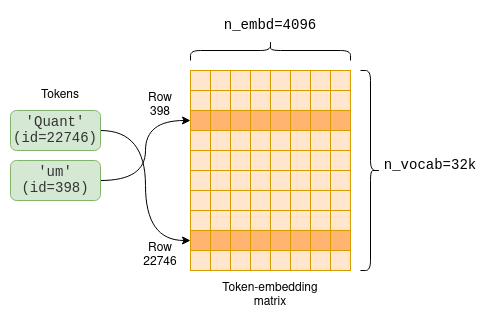
The first part of the computation graph extracts the relevant rows from the token-embedding matrix for each token:

// llama.cpp (simplified)static struct ggml_cgraph * llm_build_llama(/* ... */) {    // ...    struct ggml_tensor * inp_tokens = ggml_new_tensor_1d(ctx0, GGML_TYPE_I32, n_tokens);    memcpy(        inp_tokens->data,        tokens,        n_tokens * ggml_element_size(inp_tokens));    inpL = ggml_get_rows(ctx0, model.tok_embeddings, inp_tokens);}//

The code first creates a new one-dimensional tensor of integers, called inp_tokens, to hold the numerical tokens.Then, it copies the token values into this tensor’s data pointer.Last, it creates a new GGML_OP_GET_ROWS tensor operation combining the token-embedding matrix model.tok_embeddings with our tokens.

This operation, when later computed, pulls rows from the embeddings matrix as shown in the diagram above to create a new n_tokens x n_embd matrix containing only the embeddings for our tokens in their original order:

The Transformer

The main part of the computation graph is called the Transformer.The Transformer is a neural network architecture that is the core of the LLM, and performs the main inference logic.In the following section we will explore some key aspects of the transformer from an engineering perspective, focusing on the self-attention mechanism.If you want to gain an understanding of the intuition behind the Transformer’s architecture instead, I recommend reading The Illustrated Transformer².

Self-attention

We first zoom in to look at what self-attention is; after which we will zoom back out to see how it fits within the overall Transformer architecture³.

Self-attention is a mechanism that takes a sequence of tokens and produces a compact vector representation of that sequence, taking into account the relationships between the tokens.It is the only place within the LLM architecture where the relationships between the tokens are computed. Therefore, it forms the core of language comprehension, which entails understanding word relationships.Since it involves cross-token computations, it is also the most interesting place from an engineering perspective, as the computations can grow quite large, especially for longer sequences.

The input to the self-attention mechanism is the n_tokens x n_embd embedding matrix, with each row, or vector, representing an indivisual token⁴.Each of these vectors is then transformed into three distinct vectors, called “key”, “query” and “value” vectors.The transformation is achieved by multiplying the embedding vector of each token with the fixed wk, wq and wv matrices, which are part of the model parameters:

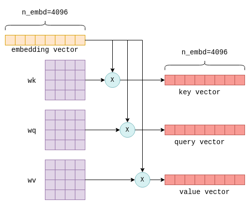
This process is repeated for every token, i.e. n_tokens times. Theoretically, this could be done in a loop but for efficiency all rows are transformed in a single operation using matrix multiplication, which does exactly that. The relevant code looks as follows:

// llama.cpp (simplified to remove use of cache)// `cur` contains the input to the self-attention mechanismstruct ggml_tensor * K = ggml_mul_mat(ctx0,    model.layers[il].wk, cur);struct ggml_tensor * Q = ggml_mul_mat(ctx0,    model.layers[il].wq, cur);struct ggml_tensor * V = ggml_mul_mat(ctx0,    model.layers[il].wv, cur);

We end up with K,Q and V: Three matrices, also of size n_tokens x n_embd, with the key, query and value vectors for each token stacked together.

The next step of self-attention involves multiplying the matrix Q, which contains the stacked query vectors, with the transpose of the matrix K, which contains the stacked key vectors.For those less familiar with matrix operations, this operation essentially calculates a joint score for each pair of query and key vectors.We will use the notation S(i,j) to denote the score of query i with key j.

This process yield n_tokens^2 scores, one for each query-key pair, packed within a single matrix called KQ.This matrix is subsequently masked to remove the entries above the diagonal:

The masking operation is a critical step. For each token it retains scores only with its preceeding tokens.During the training phase, this constraint ensures that the LLM learns to predict tokens based solely on past tokens, rather than future ones.Moreover, as we’ll explore in more detail later, it allows for significant optimizations when predicting future tokens.

The last step of self-attention involves multiplying the masked scoring KQ_masked with the value vectors from before⁵.Such a matrix multiplication operation creates a weighted sum of the value vectors of all preceeding tokens, where the weights are the scores S(i,j).For example, for the fourth token ics it creates a weighted sum of the value vectors of Quant, um, ▁mechan and ics with the weights S(3,0) to S(3,3), which themselves were calculated from the query vector of ics and all preceeding key vectors.

The KQV matrix concludes the self-attention mechanism. The relevant code implementing self-attention was already presented before in the context of general tensor computations, but now you are better equipped fully understand it.

The layers of the Transformer

Self-attention is one of the components in what are called the layers of the transformer.Each layer, in addition to the self-attention mechanism, contains multiple other tensor operations, mostly matrix addition, multiplication and activation that are part of a feed-forward neural network.We will not explore these more in detail, but just note the following facts:

• Large, fixed, parameter matrices are used in the feed-forward network. In LLaMA-7B, their sizes are n_embd x n_ff = 4096 x 11008.
• Besides self-attention, all other operations can be thought of as being carried row-by-row, or token-by-token. As mentioned before, only self-attention contains cross-token calculations. This will be important later when discussing the kv-cache.
• The input and output are always of size n_tokens x n_embd: One row for each token, each the size of the model’s dimension.

For completeness I included a diagram of a single Transformer layer in LLaMA-7B. Note that the exact architecture will most likely vary slightly in future models.

In a Transformer architecture there are multiple layers. For example, in LLaMA-7B there are n_layers=32 layers.The layers are identical except that each has its own set of parameter matrices (e.g. its own wk, wq and wv matrices for the self-attention mechanism).The first layer’s input is the embedding matrix as described above. The first layer’s output is then used as the input to the second layer and so on.We can think of it as if each layer produces a list of embeddings, but each embedding no longer tied directly to a single token but rather to some kind of more complex understanding of token relationships.

Calculating the logits

The final step of the Transformer involves the computation of logits.A logit is a floating-point number that represents the probability that a particular token is the “correct” next token.The higher the value of the logit, the more likely it is that the corresponding token is the “correct” one.

The logits are calculated by multiplying the output of the last Transformer layer with a fixed n_embd x n_vocab parameter matrix (also called output in llama.cpp).This operation results in a logit for each token in our vocabulary. For example, in LLaMA, it results in n_vocab=32000 logits:

The logits are the Transformer’s output and tell us what the most likely next tokens are. By this all the tensor computations are concluded.The following simplified and commented version of the llm_build_llama() function summarizes all steps which were described in this section:

// llama.cpp (simplified and commented)static struct ggml_cgraph * llm_build_llama(         llama_context & lctx,     const llama_token * tokens,                   int   n_tokens,                   int   n_past) {    ggml_cgraph * gf = ggml_new_graph(ctx0);    struct ggml_tensor * cur;    struct ggml_tensor * inpL;    // Create a tensor to hold the tokens.    struct ggml_tensor * inp_tokens = ggml_new_tensor_1d(ctx0, GGML_TYPE_I32, N);    // Copy the tokens into the tensor    memcpy(        inp_tokens->data,        tokens,        n_tokens * ggml_element_size(inp_tokens));    // Create the embedding matrix.    inpL = ggml_get_rows(ctx0,        model.tok_embeddings,        inp_tokens);    // Iteratively apply all layers.    for (int il = 0; il < n_layer; ++il) {        struct ggml_tensor * K = ggml_mul_mat(ctx0, model.layers[il].wk, cur);        struct ggml_tensor * Q = ggml_mul_mat(ctx0, model.layers[il].wq, cur);        struct ggml_tensor * V = ggml_mul_mat(ctx0, model.layers[il].wv, cur);        struct ggml_tensor * KQ = ggml_mul_mat(ctx0, K, Q);        struct ggml_tensor * KQ_scaled = ggml_scale_inplace(ctx0, KQ, KQ_scale);        struct ggml_tensor * KQ_masked = ggml_diag_mask_inf_inplace(ctx0,            KQ_scaled, n_past);        struct ggml_tensor * KQ_soft_max = ggml_soft_max_inplace(ctx0, KQ_masked);        struct ggml_tensor * KQV = ggml_mul_mat(ctx0, V, KQ_soft_max);        // Run feed-forward network.        // Produces `cur`.        // ...        // input for next layer        inpL = cur;    }    cur = inpL;    // Calculate logits from last layer's output.    cur = ggml_mul_mat(ctx0, model.output, cur);    // Build and return the computation graph.    ggml_build_forward_expand(gf, cur);    return gf;}

To actually performn inference, the computation graph returned by this function is computed, using ggml_graph_compute() as described previously.The logits are then copied out from the last tensor’s data pointer into an array of floats, ready for the next step called sampling.

Sampling

With the list of logits in hand, the next step is to choose the next token based on them. This process is called sampling. There are multiple sampling methods available, suitable for different use cases. In this section we will cover two basic sampling methods, with more advanced sampling methods like grammar sampling reserved for future posts.

Greedy sampling

Greedy sampling is a straightforward approach that selects the token with the highest logit associated with it.

For our example prompt, the following tokens have the highest logits:

token	logit
▁describes	18.990
▁provides	17.871
▁explains	17.403
▁de	16.361
▁gives	15.007

Therefore, greedy sampling will deterministically choose ▁describes as the next token.Greedy sampling is most useful when deterministic outputs are required when re-evaluating identical prompts.

Temperature sampling

Temperature sampling is probabilistic, meaning that the same prompt might produce different outputs when re-evaluated.It uses a parameter called temperature which is a floating-point value between 0 and 1 and affects the randomness of the result. The process goes as follows:

1. The logits are sorted from high to low and normalized using a softmax function to ensure that they all sum to 1. This transformation converts each logit into a probability.
2. A threshold (set to 0.95 by default) is applied, retaining only the top tokens such that their cumulative probability remains below the threshold. This step effectively removes low-probability tokens, preventing “bad” or “incorrect” tokens from being rarely sampled.
3. The remaining logits are divided by the temperature parameter and normalized again such that they all sum to 1 and represent probabilities.
4. A token is randomly sampled based on these probabilities. For example, in our prompt, the token ▁describes has a probability of p=0.6, meaning that it will be chosen approximately 60% of the time. Upon re-evaluation, different tokens may be chosen.

The temperature parameter in step 3 serves to either increase or decrease randomness.Lower temperature values suppress lower probability tokens, making it more likely that the same tokens will be chosen on re-evaluation. Therefore, lower temperature values decrease randomness.In contrast, higher temperature values tend to “flatten” the probability distribution, emphasizing lower probability tokens. This increases the likelihood that each re-evaluation will result in different tokens, increasing randomness.

Sampling a token concludes a full iteration of the LLM.After the initial token is sampled, it is added to the list of tokens, and the entire process runs again.The output iteratively becomes the input to the LLM, increasing by one token each iteration.

Theoretically, subsequent iterations can be carried out identically. However, to address performance degradation as the list of tokens grows, certain optimizations are employed. These will be covered next.

Optimizing inference

The self-attention stage of the Transformer can become a performance bottleneck as the list of input tokens to the LLM grows.A longer list of tokens means that larger matrices are multiplied together. Each matrix multiplication consists of many smaller numerical operations, known as floating-point operations, which are constrained by the GPU’s floating-point-operations-per-second capacity (flops).In the Transformer Inference Arithmetic, it is calculated that for a 52B parameter model, on an A100 GPU, performance starts to degrade at 208 tokens due to excessive flops.The most commonly employed optimization technique to solve this bottleneck is known as the kv cache.

The KV cache

To recap, each token has an associated embedding vector, which is further transformed into key and value vectors by multiplying it with the parameter matrices wk and wv.The kv cache is a cache for these key and value vectors.By caching them, we save the floating point operations required for re-calculating them on each iteration.

The cache works as follows:

• During the initial iteration, the key and value vectors are computed for all tokens, as previously described, and then saved into the kv cache.
• In subsequent iterations, only the key and value vectors for the newest token need to be calculated.The cached k-v vectors, together with the k-v vectors for the new token, are concatenated together to form the K and V matrices.This saves recalculating the k-v vectors for all previous tokens, which can be significant.

The ability to utilize a cache for key and value vectors arises from the fact that these vectors remain identical between iterations.For example, if we first process four tokens, and then five tokens, with the initial four unchanged, then the first four key and value vectors will remain identical between the first and the second iteration.As a result, there’s no need to recalculate key and value vectors for the first four tokens in the second iteration.

This principle holds true for all layers within the Transformer, not just the first one.In all layers, the key and value vectors for each token are solely dependent on previous tokens.Therefore, as new tokens are appended in subsequent iterations, the key and value vectors for existing tokens remain the same.

For the first layer, this concept is relatively straightforward to verify:the key vector of a token is determined by multiplying the token’s fixed embedding with the fixed wk parameter matrix.Thus, it remains unchanged in subsequent iterations, regardless of the additional tokens introduced.The same rationale applies to the value vector.

For the second layer and beyond, this principle is a bit less obvious but still holds true.To understand why, consider the first layer’s KQV matrix, the output of the self-attention stage.Each row in the KQV matrix is a weighted sum that depends on:

• Value vectors of previous tokens.
• Scores calculated from key vectors of previous tokens.

Therefore each row in KQV solely relies on previous tokens.This matrix, following a few additional row-based operations, serves as the input to the second layer.This implies that the second layer’s input will remain unchanged in future iterations, except for the addition of new rows.Inductively, the same logic extends to the rest of the layers.

Further optimizing subsequent iterations

You might wonder why we don’t cache the query vectors as well, considering we cache the key and value vectors.The answer is that in fact, except for the query vector of the current token, query vectors for previous tokens are unnecessary in subsequent iterations.With the kv cache in place, we can actually feed the self-attention mechanism only with the latest token’s query vector.This query vector is multiplied with the cached K matrix to calculate the joint scores of the last token and all previous tokens.Then, it is multiplied with the cached V matrix to calculate only the latest row of the KQV matrix.In fact, across all layers, we now pass 1 x n_embd -sized vectors instead of the n_token x n_embd matrices calculated in the first iteration.To illustrate this, compare the following diagram, showing a later iteration, with the previous one:

This process repeats across all layers, utilizing each layer’s kv cache.As a result, the Transformer’s output in this case is a single vector of n_vocab logits predicting the next token.

With this optimization we save floating point operations of calculating unnecessary rows in KQ and KQV, which can become quite significant as the list of tokens grows in size.

The KV cache in practice

We can dive into llama.cpp code to see how the kv cache is implemented in practice.Unsurprisingly maybe, it is built using tensors, one for key vectors and one for value vectors:

// llama.cpp (simplified)struct llama_kv_cache {    // cache of key vectors    struct ggml_tensor * k = NULL;    // cache of value vectors    struct ggml_tensor * v = NULL;    int n; // number of tokens currently in the cache};

When the cache is initialized, enough space is allocated to hold 512 key and value vectors for each layer:

// llama.cpp (simplified)// n_ctx = 512 by defaultstatic bool llama_kv_cache_init(    struct llama_kv_cache & cache,    ggml_type   wtype,    int   n_ctx) {    // Allocate enough elements to hold n_ctx vectors for each layer.    const int64_t n_elements = n_embd*n_layer*n_ctx;    cache.k = ggml_new_tensor_1d(cache.ctx, wtype, n_elements);    cache.v = ggml_new_tensor_1d(cache.ctx, wtype, n_elements);    // ...}

Recall that during inference, the computation graph is built using the function llm_build_llama().This function has a parameter called n_past that we ignored before.In the first iteration, the n_tokens parameter contains the number of tokens and n_past is set to 0.In subsequent iterations, n_tokens is set to 1 because only the latest token is processed, and n_past contains the number of past tokens. n_past is then used to pull the correct number of key and value vectors from the kv cache.

The relevant part from this function is shown here, utilizing the cache for calculating the K matrix.I simplified it slightly to ignore the multi-head attention and added comments for each step:

// llama.cpp (simplified and commented)static struct ggml_cgraph * llm_build_llama(    llama_context & lctx,    const llama_token * tokens,    int   n_tokens,    int   n_past) {    // ...    // Iteratively apply all layers.    for (int il = 0; il < n_layer; ++il) {         // Compute the key vector of the latest token.         struct ggml_tensor * Kcur = ggml_mul_mat(ctx0, model.layers[il].wk, cur);         // Build a view of size n_embd into an empty slot in the cache.         struct ggml_tensor * k = ggml_view_1d(            ctx0,            kv_cache.k,            // size            n_tokens*n_embd,            // offset            (ggml_element_size(kv_cache.k)*n_embd) * (il*n_ctx + n_past)         );         // Copy latest token's k vector into the empty cache slot.         ggml_cpy(ctx0, Kcur, k);         // Form the K matrix by taking a view of the cache.         struct ggml_tensor * K =             ggml_view_2d(ctx0,                 kv_self.k,                 // row size                 n_embd,                 // number of rows                 n_past + n_tokens,                 // stride                 ggml_element_size(kv_self.k) * n_embd,                 // cache offset                 ggml_element_size(kv_self.k) * n_embd * n_ctx * il);    }}

First, the new key vector is calculated.Then, n_past is used to find the next empty slot in the cache, and the new key vector is copied there.Last, the matrix K is formed by taking a view into the cache with the correct number of tokens (n_past + n_tokens).

The kv cache is the basis for LLM inference optimization.It’s worth noting that the version implemented in llama.cpp (as of this writing) and presented here is not the most optimal one.For instance, it allocates a lot of memory in advance to hold the maximum number of key and value vectors supported (512 in this case).More advanced implementations, such as vLLM, aim to enhance memory usage efficiency and may offer further performance improvement. These advanced techniques are reserved for future posts.Moreover, as this field moves forward at lightning speeds, there are likely to be new and improved optimization techniques in the future.

Concluding

This post covered quite a lot of ground and should give you a basic understanding of the full process of LLM inference.With this knowledge you can get around more advanced resources:

• LLM parameter counting and Transformer Inference Arithmetic analyze LLM performance in depth.
• vLLM is a library for managing the kv cache memory more efficiently.
• Continuous batching is an optimization technique to batch multiple LLM prompts together.

I also hope to cover the internals of more advanced topics in future posts. Some options include:

• Quantized models.
• Fine-tuned LLMs using LoRA.
• Various attention mechanisms (Multi-head attention, Grouped-query attention and Sliding window attention).
• LLM request batching.
• Grammar sampling.

Stay tuned!

---

Footnotes

Footnotes

1. ggml also provides ggml_build_backward() that computes gradients in a backward manner from output to input. This is used for backpropagation only during model training, and never in inference. ↩

2. The article describes an encoder-decoder model. LLaMA is a decoder-only model, because it only predicts one token at a time. But the core concpets are the same. ↩

3. For simplicity I have chosen to describe here a single-head self-attention mechanism. LLaMA uses a multi-head self-attention mechanism. Except for making the tensor operations a bit more complicated, it has no implications for the core ideas presented in this section. ↩

4. To be precise, the embeddings first undergo a normalization operation that scales their values. We ignore it as it does not affect the core ideas presented. ↩

5. The scores also undergo a softmax operation, which scales them so that each row of scores sums of to 1. ↩

我们从研究这个过程的整体流程开始。从核心来看，LLM每次只预测一个词元。通过反复将LLM模型应用于相同的提示，并将之前的输出词元附加到提示上，实现生成完整句子（或更多）。这种类型的模型被称为自回归模型。因此，我们的关注点主要是生成单个标记，如下

(从用户提示生成单个词元的完整流程包括多个阶段，例如分词、嵌入、Transformer神经网络和采样)

上图的流程描述如下：

1. 分词器将提示分割成一个词元列表。根据模型的词汇表，某些单词可能会被拆分成多个词元。每个词元由一个唯一的数字表示；
2. 每个数值标记都会转换成一个嵌入。嵌入是一个固定大小的向量，这种方式来表征词元便于LLM处理。所有的嵌入一起形成一个嵌入矩阵；
3. 嵌入矩阵作为输入送入Transformer。Transformer是一个神经网络，是LLM的核心。Transformer由多个层组成的链条构成。每层接收一个输入矩阵，并使用模型参数对其进行各种数学运算，最显著的是自注意力机制。该层的输出被用作下一层的输入；
4. 一个最终的神经网络将Transformer的输出转换成logits。每个可能的下一个词元都有一个对应的logits，表示该词元是句子的“正确”延续的概率；
5. 从logits列表中选择下一个词元时，会使用某种抽样技术从列表中选取一个使用；
6. 选择的词元作为输出返回。要继续生成词元，则将所选词元附加到步骤1中的词元列表中，并重复该过程，直到生成所需数量的词元，或者LLM发出一个特殊的结束流（EOS）标记。

一、llama.cpp大模型推理框架交叉编译<推理框架和后端均为CPU>

1): 指定CPU架构

     llama.cpp-b4667/CMakeLists.txt

     添加CPU类型:

     set( CMAKE_SYSTEM_PROCESSOR   aarch64)

2): cmake   -DGGML_NATIVE=OFF     -DGGML_CPU_ARM_ARCH=armv8-a  -DBUILD_SHARED_LIBS=OFF  ../

问题：

1、如果出现如下错误:

则可以升级当前的交叉编译器，即可解决。比如用gcc-arm-10.3-2021.07-x86_64-aarch64-none-linux-gnu.tar.xz，就没有这个问题.

在网上还看到有其它的方法：

ggml/src/ggml-blas/CMakeLists.txt 文件添加如下内容:

target_compile_options(${GGML_CPU_NAME} PRIVATE -flax-vector-conversions)

解决办法:

cmake   -DGGML_NATIVE=OFF     -DGGML_CPU_ARM_ARCH=armv8-a     ../