./llama-cli  -cnv  --chat-template deepseek3   -m   /home/flmxi/Downloads/llama-b4667-bin-ubuntu-x64/deepseekR1_1.5B_FP16.gguf

将safetensors格式转为gguf格式:

1、下载llama (C/C++ 大模型推理框架)

    https://github.com/ggerganov/llama.cpp, 利用llama自带的转换脚本: convert_hf_to_gguf.py

2、准备safetensors模型的三个文件,并且放在同一个目录下, 比如: ~/model_demo/

    (1): xxx.safetensors

    (2): config.json

    (3): tokenizer.json

3、利用python 工具转换

    python3  convert_hf_to_gguf.py   ~/model_demo/   --verbose  --outtype f16

github:

 https://github.com/ggerganov/llama.cpp

https://github.com/ggml-org/llama.cpp

Yolov8 developed by ultralytics is a state of the art model which can be used for both real time object detection and instance segmentation.

The model requires data in yolo format to perform these operations. Ultralytics has provided the code to convert the labels from yolo object detection format to yolo segmentation format.

We can leverage the power of SAM(segment anything model) model to generate the segmentation masks for a dataset containing detection labels(bounding boxes ) in YOLO format. This is a powerful approach to address the challenge of creating segmentation masks from a dataset with only detection labels.

Object Detection Dataset

The Yolo format of a dataset will be in the ‘.txt’ format. Each image has a corresponding text file. For object detection, the text file contains data in the format which looks like the one below. Each of the line in the text file represents an object in the image.Given below is an example of a line in the text file, where the very first digit represents the class label. The next four digits represent the center x-coordinate, center y-coordinate, width and height of the bounding box that is drawn around the object.

Class id, center x, center y, width, height

0 0.8731971153846154 0.3040865384615385 0.056490384615384616 0.057692307692307696

Instance Segmentation Dataset

For each image in the dataset, YoloV8 stores the instance segmentation data in a text file. Each line in the textfile represents an object in that particular image. The model requires an encoded mask or a binary mask or a set of polygon points that outlines the shape of the object.Below is an example of a line in the text file that represents the object in an image with the very first digit representing the class id, followed by the polygon points that outlines the object.

Class id, x1, y1, x2, y2, x3, y3, x4, y4,…

0 0.798077 0.384615 0.798077 0.387019 0.799279 0.388221 0.799279 0.389423 0.798077 0.390625 0.796875 0.390625 0.795673 0.391827 0.790865 0.391827 0.794471 0.395433 0.794471 

Converting bounding boxes to segment

As a first step, let’s organize our data folders in the following structure. Create a folder called ‘seg_labels’ inside the image_dir to save the segmentation labels. So the final folder structure looks like the one below.

image_dir

├── images

│   ├── 1.jpg

│   ├── ...

│   └── n.jpg

├── labels

│   ├── 1.txt

│   ├── ...

│   └── n.txt

└── seg_labels

The code to convert the Yolo Bounding Boxes to segmentation format is provided by the ultralytics here. To start, with you have to first install the dependencies.

!pip install opencv-python ultralytics numpy

Then import all the required libraries.

from tqdm import tqdm

import ultralytics

from ultralytics import SAM

from ultralytics.data import YOLODataset

from ultralytics.utils import LOGGER

from ultralytics.utils.ops import xywh2xyxy

from pathlib import Path

import cv2

import os

Define a function to convert bounding boxes to segmentation format. This function is adapted from the Ultralytics website.

The function first checks if the segmentation labels already exist. If they do not, it checks for the presence of detection labels. If detection labels are present, the function generates segmentation labels using the SAM model and saves them into a new directory for segmentation labels.

def yolo_bbox2segment(im_dir, save_dir=None, sam_model="sam_b.pt"):

    """

    Converts existing object detection dataset (bounding boxes) to segmentation dataset or oriented bounding box (OBB)

    in YOLO format. Generates segmentation data using SAM auto-annotator as needed.



    Args:

        im_dir (str | Path): Path to image directory to convert.

        save_dir (str | Path): Path to save the generated labels, labels will be saved

            into `labels-segment` in the same directory level of `im_dir` if save_dir is None. Default: None.

        sam_model (str): Segmentation model to use for intermediate segmentation data; optional.



    """



    # NOTE: add placeholder to pass class index check

    dataset = YOLODataset(im_dir, data=dict(names=list(range(1000))))



    if len(dataset.labels[0]["segments"]) > 0:  # if it's segment data

        LOGGER.info("Segmentation labels detected, no need to generate new ones!")

        return

    LOGGER.info("Detection labels detected, generating segment labels by SAM model!")

    sam_model = SAM(sam_model)

    

    #process YOLO labels and generate segmentation masks using the SAM model

    for l in tqdm(dataset.labels, total=len(dataset.labels), desc="Generating segment labels"):

        h, w = l["shape"]

        boxes = l["bboxes"]

        if len(boxes) == 0:  # skip empty labels

            continue

        boxes[:, [0, 2]] *= w

        boxes[:, [1, 3]] *= h

        im = cv2.imread(l["im_file"])

        sam_results = sam_model(im, bboxes=xywh2xyxy(boxes), verbose=False, save=False)

        l["segments"] = sam_results[0].masks.xyn



    save_dir = Path(save_dir) if save_dir else Path(im_dir).parent / "labels-segment"

    save_dir.mkdir(parents=True, exist_ok=True)

    

    # Saves segmentation masks and class labels to text files for each image

    for l in dataset.labels:

        texts = []

        lb_name = Path(l["im_file"]).with_suffix(".txt").name

        txt_file = save_dir / lb_name

        cls = l["cls"]

        for i, s in enumerate(l["segments"]):

            line = (int(cls[i]), *s.reshape(-1))

            texts.append(("%g " * len(line)).rstrip() % line)

        if texts:

            with open(txt_file, "a") as f:

                f.writelines(text + "\n" for text in texts)



    LOGGER.info(f"Generated segment labels saved in {save_dir}")

Download the sam model in the next step.

!wget https://github.com/ultralytics/assets/releases/download/v8.2.0/sam_b.pt

Finally, call the function to perform the conversion. Replace the values with your path to directories and models.

yolo_bbox2segment('{path to image_dir}', save_dir='{path to image_dir//seg_labels}', sam_model='{path to sam_b.pt}')

Thats all and the generated segmentation dataset will be available in the save_dir. The final folder structure looks like the one below.

image_dir

├── images

│   ├── 1.jpg

│   ├── ...

│   └── n.jpg

├── labels

│   ├── 1.txt

│   ├── ...

│   └── n.txt

└── seg_labels

    ├── 1.txt

    ├── ...

    └── n.txt

Reference:
converter — Ultralytics YOLOv8 Docs

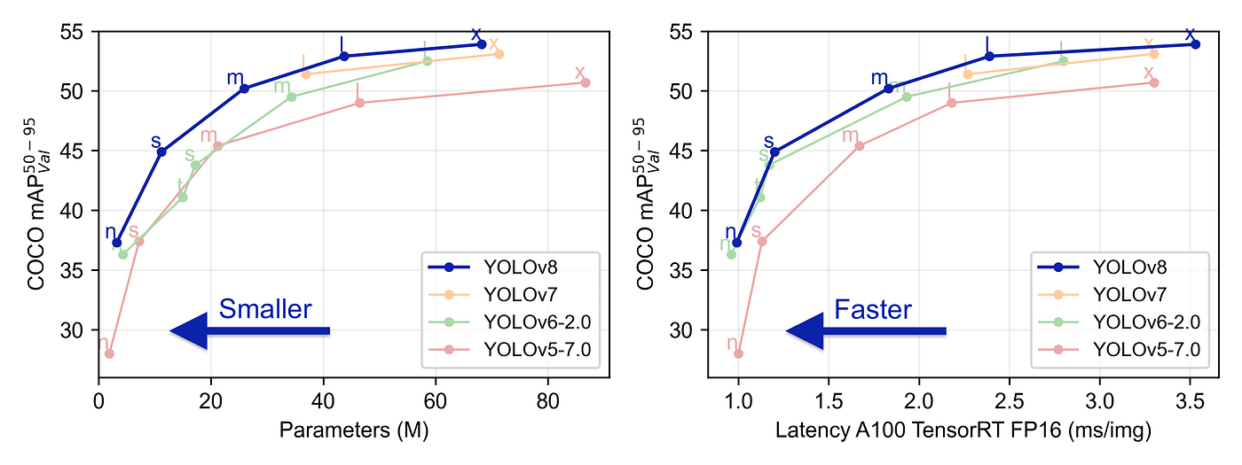
YOLOv8 was launched on January 10th, 2023. And as of this moment, this is the state-of-the-art model for classification, detection, and segmentation tasks in the computer vision world. The model outperforms all known models both in terms of accuracy and execution time.

The ultralytics team did a really good job in making this model easier to use compared to all the previous YOLO models — you don’t even have to clone the git repository anymore!

Creating the Image Dataset

In this post, I created a very simple example of all you need to do to train YOLOv8 on your data, specifically for a segmentation task. The dataset is small and “easy to learn” for the model, on purpose, so that we would be able to get satisfying results after training for only a few seconds on a simple CPU.

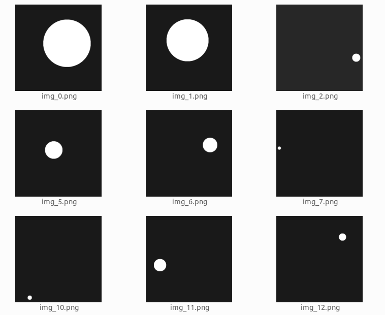
We will create a dataset of white circles with a black background. The circles will be of varying sizes. We will train a model that segments the circles inside the image.

This is what the dataset looks like:

The dataset was generated using the following code:

import numpy as np

from PIL import Image

from skimage import draw

import random

from pathlib import Path



def create_image(path, img_size, min_radius):

    path.parent.mkdir( parents=True, exist_ok=True )

    

    arr = np.zeros((img_size, img_size)).astype(np.uint8)

    center_x = random.randint(min_radius, (img_size-min_radius))

    center_y = random.randint(min_radius, (img_size-min_radius))

    max_radius = min(center_x, center_y, img_size - center_x, img_size - center_y)

    radius = random.randint(min_radius, max_radius)



    row_indxs, column_idxs = draw.ellipse(center_x, center_y, radius, radius, shape=arr.shape)

    

    arr[row_indxs, column_idxs] = 255



    im = Image.fromarray(arr)

    im.save(path)



def create_images(data_root_path, train_num, val_num, test_num, img_size=640, min_radius=10):

    data_root_path = Path(data_root_path)

    

    for i in range(train_num):

        create_image(data_root_path / 'train' / 'images' / f'img_{i}.png', img_size, min_radius)

        

    for i in range(val_num):

        create_image(data_root_path / 'val' / 'images' / f'img_{i}.png', img_size, min_radius)

        

    for i in range(test_num):

        create_image(data_root_path / 'test' / 'images' / f'img_{i}.png', img_size, min_radius)



create_images('datasets', train_num=120, val_num=40, test_num=40, img_size=120, min_radius=10)

Creating Labels

Now that we have an image dataset, we need to create labels for the images. Usually, we would need to do some manual work for this, but because the dataset we created is very simple, it is pretty easy to create code that generates labels for us:

from rasterio import features



def create_label(image_path, label_path):

    arr = np.asarray(Image.open(image_path))



    # There may be a better way to do it, but this is what I have found so far

    cords = list(features.shapes(arr, mask=(arr >0)))[0][0]['coordinates'][0]

    label_line = '0 ' + ' '.join([f'{int(cord[0])/arr.shape[0]} {int(cord[1])/arr.shape[1]}' for cord in cords])



    label_path.parent.mkdir( parents=True, exist_ok=True )

    with label_path.open('w') as f:

        f.write(label_line)



for images_dir_path in [Path(f'datasets/{x}/images') for x in ['train', 'val', 'test']]:

    for img_path in images_dir_path.iterdir():

        label_path = img_path.parent.parent / 'labels' / f'{img_path.stem}.txt'

        label_line = create_label(img_path, label_path)

Here is an example of a label file content:

0 0.0767 0.08433 0.1417 0.08433 0.1417 0.0917 0.15843 0.0917 0.15843 0.1 0.1766 0.1 0.1766 0.10844 0.175 0.10844 0.175 0.1177 0.18432 0.1177 0.18432 0.14333 0.1918 0.14333 0.1918 0.20844 0.18432 0.20844 0.18432 0.225 0.175 0.225 0.175 0.24334 0.1766 0.24334 0.1766 0.2417 0.15843 0.2417 0.15843 0.25 0.1417 0.25 0.1417 0.25846 0.0767 0.25846 0.0767 0.25 0.05 0.25 0.05 0.2417 0.04174 0.2417 0.04174 0.24334 0.04333 0.24334 0.04333 0.225 0.025 0.225 0.025 0.20844 0.01766 0.20844 0.01766 0.14333 0.025 0.14333 0.025 0.1177 0.04333 0.1177 0.04333 0.10844 0.04174 0.10844 0.04174 0.1 0.05 0.1 0.05 0.0917 0.0767 0.0917 0.0767 0.08433

The label corresponds to this image:

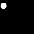
The label content is only a single text line. We have only one object (circle) in each image, and each object is represented by a line in the file. If you have more than one object in each image, you should create a line for each labeled object.

The first 0 represents the class type of the label. Because we have only one class type (a circle) we always have 0. If you have more than one class in your data, you should map each class to a number ( 0, 1, 2…) and use this number in the label file.

All the other numbers represent the coordinates of the bounding polygon of the labeled object. The format is <x1 y1 x2 y2 x3 y3…> and the coordinates are relative to the size of the image —you should normalize the coordinates to a 1x1 image size. For example, if there is a point (15, 75) and the image size is 120x120 the normalized point is (15/120, 75/120) = (0.125, 0.625).

It is always confusing when dealing with image libraries to get the correct directionality of the coordinates. So to make this clear, for YOLO, the X coordinate goes from left to right, and the Y coordinate goes from top to bottom.

The YAML Configuration

We have the images and the labels. Now we need to create a YAML file with the dataset configuration:

yaml_content = f'''

train: train/images

val: val/images

test: test/images



names: ['circle']

    '''

    

with Path('data.yaml').open('w') as f:

    f.write(yaml_content)

Pay attention that if you have more object class types, you need to add them here in the names array, in the same order you ordered them in the label files. The first is 0, the second is 1, etc…

Dataset File Structure

Let's see the file structure we created, using the Linux tree command:

tree .

data.yaml

datasets/

├── test

│   ├── images

│   │   ├── img_0.png

│   │   ├── img_1.png

│   │   ├── img_2.png

│   │   ├── ...

│   └── labels

│       ├── img_0.txt

│       ├── img_1.txt

│       ├── img_2.txt

│       ├── ...

├── train

│   ├── images

│   │   ├── img_0.png

│   │   ├── img_1.png

│   │   ├── img_2.png

│   │   ├── ...

│   └── labels

│       ├── img_0.txt

│       ├── img_1.txt

│       ├── img_2.txt

│       ├── ...

|── val

|   ├── images

│   │   ├── img_0.png

│   │   ├── img_1.png

│   │   ├── img_2.png

│   │   ├── ...

|   └── labels

│       ├── img_0.txt

│       ├── img_1.txt

│       ├── img_2.txt

│       ├── ...

Training The Model

Now that we have the images and the labels, we can start training the model. So first of all let's install the package:

pip install ultralytics==8.0.38

The ultralytics library changes pretty fast and sometimes breaks the API, so I prefer to stick with one version. The below code depends on version 8.0.38 (the newest version at the time I write those words). If you upgrade to a newer version, maybe you will need to do some code adaptations to make it work.

And start the training:

from ultralytics import YOLO



model = YOLO("yolov8n-seg.pt")



results = model.train(

        batch=8,

        device="cpu",

        data="data.yaml",

        epochs=7,

        imgsz=120,

    )

For the simplicity of this post, I use the nano model (yolov8n-seg), I train it only on the CPU, with only 7 epochs. The training took just a few seconds on my laptop.

For more information about the parameters that can be used to train the model, you can check this.

Understanding the Results

After the training is done you will see a line, similar to this, at the end of the output:

Results saved to runs/segment/train60

Let’s take a look at some of the results found here:

Validation labels

from IPython.display import Image as show_image

show_image(filename="runs/segment/train60/val_batch0_labels.jpg")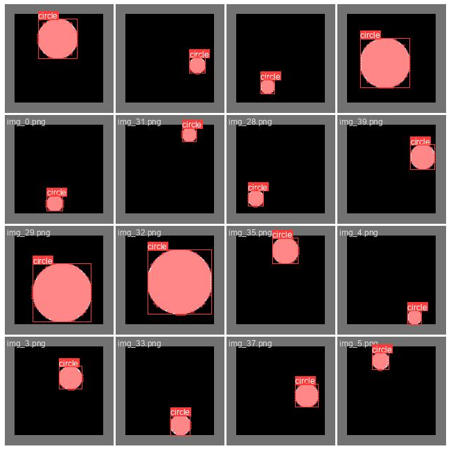

Here we can see the ground truth labels on part of the validation set. This should be almost perfectly aligned. In case you see those labels do not cover the objects well, it is highly likely that your labeling is incorrect.

Predicted validation labels

show_image(filename="runs/segment/train60/val_batch0_pred.jpg")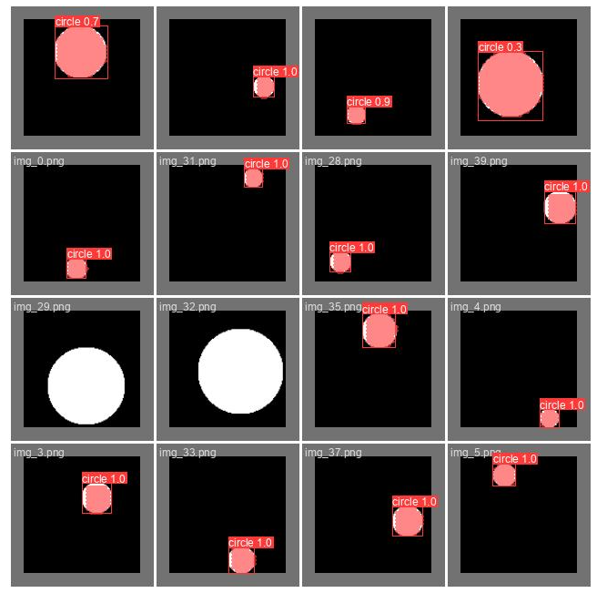

Here we can see the predictions the trained model did on part of the validation set (the same part we saw above). This can give you a feeling of how well the model performs. Pay attention that in order to create this image a confidence threshold should be chosen, the threshold used here is 0.5, which is not always the optimal one (we will discuss it later).

Precision curve

To understand this and the next charts you need to be familiar with precision and recall concepts. Here is a good explanation of how they work.

show_image(filename="runs/segment/train60/MaskP_curve.png")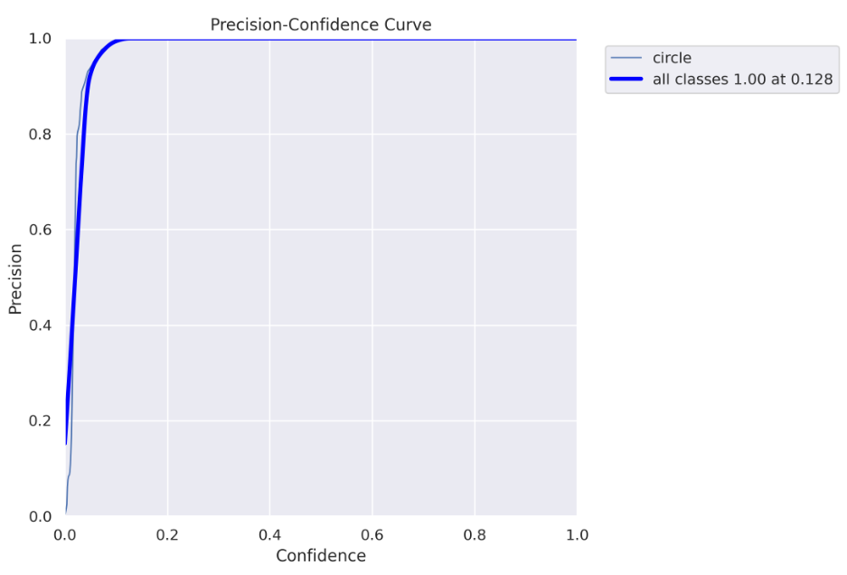

Every detected object by the model has some confidence, usually, if it is important to you to be as sure as possible when declaring “this is a circle” you will use only high confidence values (high confidence threshold). Off course, it comes with a tradeoff- you can miss some “circles”. On the other hand, if you want to “catch” as many “circles” as you can with a tradeoff that some of them are not really “circles” you would use both low and high confidence values (low confidence threshold).

The above chart (and the chart below) helps you decide which confidence threshold to use. In our case, we can see that for a threshold higher than 0.128, we get 100% precision, which means all objects are correctly predicted.

Pay attention that because we actually doing a segmentation task, there is another important threshold we need to worry about — IoU ( intersection over union), if you are not familiar with it, you can read about it here. For this chart, an IoU of 0.5 is used.

Recall curve

show_image(filename="runs/segment/train60/MaskR_curve.png")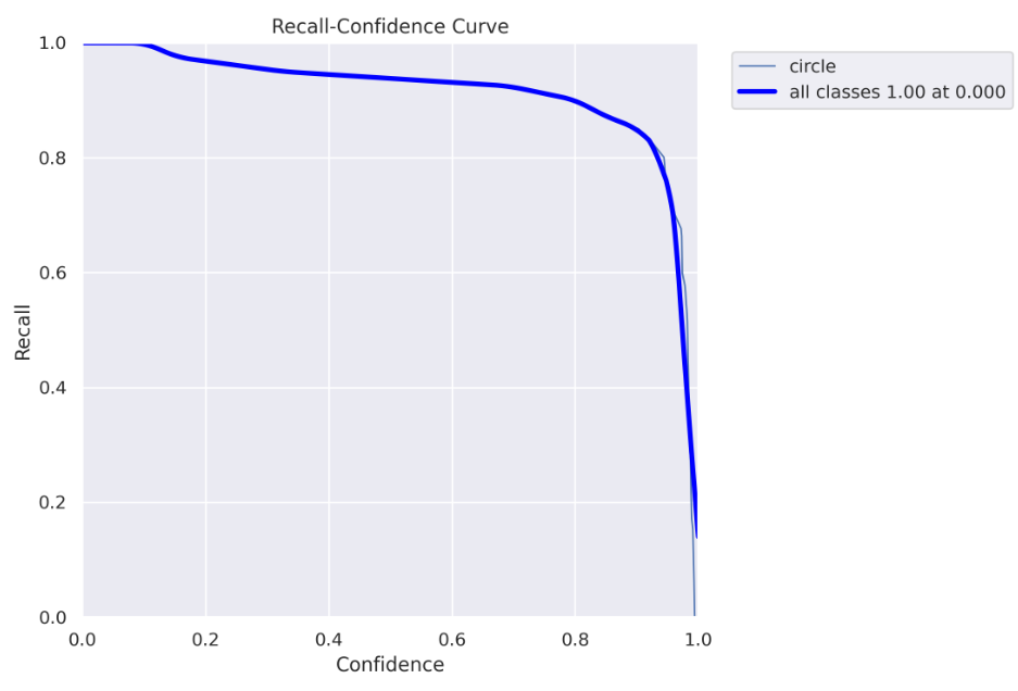

Here you can see the recall chart, as the confidence threshold values go up, the recall goes down. Which means you “catch” fewer “circles”.

Here you can see why using the 0.5 confidence threshold, in this case, is a bad idea. For a 0.5 threshold, you get about 90% recall. However, in the precision curve, we saw that for a threshold above 0.128, we get 100% precision, so we don’t need to get to 0.5, we can safely use a 0.128 threshold and get both 100% precision and almost 100% recall :)

Precision-Recall curve

Here is a good explanation of the precision-recall curve

show_image(filename="runs/segment/train60/MaskPR_curve.png")

We can see here clearly the conclusion we made before, for this model, we can get to almost 100% precision and 100% recall.

The disadvantage of this chart is that we can’t see what threshold we should use, this is why we still need the charts above.

Loss over time

show_image(filename="runs/segment/train60/results.png")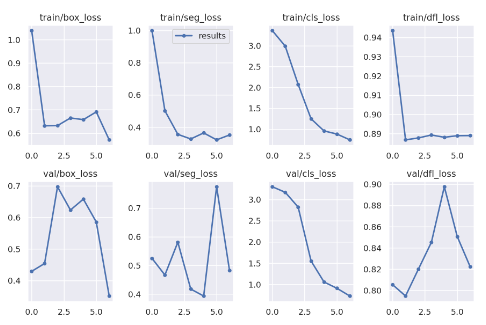

Here you can see how the different losses change during the training, and how they behave on the validation set after each epoch.

There is a lot to say about the losses, and conclusions you can make from those charts, however, it is out of the scope of this post. I just wanted to state that you can find it here :)

Using the trained model

Another thing that can be found in the result directory is the model itself. Here’s how to use the model on new images:

my_model = YOLO('runs/segment/train60/weights/best.pt')

results = list(my_model('datasets/test/images/img_5.png', conf=0.128))

result = results[0]

The results list may have multiple values, one for each detected object. Because in this example we have only one object in each image, we take the first list item.

You can see I passed here the best confidence threshold value we found before (0.128).

There are two ways to get the actual placement of the detected object in the image. Choosing the right method depends on what you intend to do with the results. I will show both ways.

result.masks.segments

[array([[    0.10156,     0.34375],

        [    0.09375,     0.35156],

        [    0.09375,     0.35937],

        [   0.078125,       0.375],

        [   0.070312,       0.375],

        [     0.0625,     0.38281],

        [    0.38281,     0.71094],

        [    0.39062,     0.71094],

        [    0.39844,     0.70312],

        [    0.39844,     0.69531],

        [    0.41406,     0.67969],

        [    0.42187,     0.67969],

        [    0.44531,     0.46875],

        [    0.42969,     0.45312],

        [    0.42969,     0.41406],

        [    0.42187,     0.40625],

        [    0.41406,     0.40625],

        [    0.39844,     0.39062],

        [    0.39844,     0.38281],

        [    0.39062,       0.375],

        [    0.38281,       0.375],

        [    0.35156,     0.34375]], dtype=float32)]

This returns the bounding polygon of the object, similar to the format we passed the labeled data.

And the second way:

result.masks.masks

tensor([[[0., 0., 0.,  ..., 0., 0., 0.],

         [0., 0., 0.,  ..., 0., 0., 0.],

         [0., 0., 0.,  ..., 0., 0., 0.],

         ...,

         [0., 0., 0.,  ..., 0., 0., 0.],

         [0., 0., 0.,  ..., 0., 0., 0.],

         [0., 0., 0.,  ..., 0., 0., 0.]]])

This returns a tensor with a shape (1, 128, 128) that represents all the pixels in the image. Pixels that are part of the object receive 1 and background pixels receive 0.

Let’s see what the mask looks like:

import torchvision.transforms as T

T.ToPILImage()(result.masks.masks).show()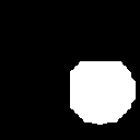

This was the original image:

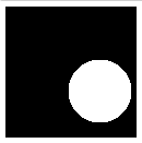
Not perfect, but good enough for many applications, and the IoU is definitely higher than 0.5.

In conclusion, the new ultralytics library is much easier to work with compared to the previous Yolo versions, especially for the segmentation task, which is now a first-class citizen. You can find Yolov5 also as part of the ultralytics new package, so if you don’t want to use the new Yolo version, which is still kind of new and experimental, you can just use the well-known yolov5:

There were some topics I didn’t cover, like the different loss functions used for the model, the architecture changes that were made to create the yolov8, and more. Feel free to comment on this post if you want more information about those topics. If there will be interest, I will maybe write another post about it.

Thanks for taking the time to read this and I hope it helped you understand the Yolov8 model training process.