Yolov8 developed by ultralytics is a state of the art model which can be used for both real time object detection and instance segmentation.

The model requires data in yolo format to perform these operations. Ultralytics has provided the code to convert the labels from yolo object detection format to yolo segmentation format.

We can leverage the power of SAM(segment anything model) model to generate the segmentation masks for a dataset containing detection labels(bounding boxes ) in YOLO format. This is a powerful approach to address the challenge of creating segmentation masks from a dataset with only detection labels.

Object Detection Dataset

The Yolo format of a dataset will be in the ‘.txt’ format. Each image has a corresponding text file. For object detection, the text file contains data in the format which looks like the one below. Each of the line in the text file represents an object in the image.Given below is an example of a line in the text file, where the very first digit represents the class label. The next four digits represent the center x-coordinate, center y-coordinate, width and height of the bounding box that is drawn around the object.

Class id, center x, center y, width, height

0 0.8731971153846154 0.3040865384615385 0.056490384615384616 0.057692307692307696

Instance Segmentation Dataset

For each image in the dataset, YoloV8 stores the instance segmentation data in a text file. Each line in the textfile represents an object in that particular image. The model requires an encoded mask or a binary mask or a set of polygon points that outlines the shape of the object.Below is an example of a line in the text file that represents the object in an image with the very first digit representing the class id, followed by the polygon points that outlines the object.

Class id, x1, y1, x2, y2, x3, y3, x4, y4,…

0 0.798077 0.384615 0.798077 0.387019 0.799279 0.388221 0.799279 0.389423 0.798077 0.390625 0.796875 0.390625 0.795673 0.391827 0.790865 0.391827 0.794471 0.395433 0.794471 

Converting bounding boxes to segment

As a first step, let’s organize our data folders in the following structure. Create a folder called ‘seg_labels’ inside the image_dir to save the segmentation labels. So the final folder structure looks like the one below.

image_dir

├── images

│   ├── 1.jpg

│   ├── ...

│   └── n.jpg

├── labels

│   ├── 1.txt

│   ├── ...

│   └── n.txt

└── seg_labels

The code to convert the Yolo Bounding Boxes to segmentation format is provided by the ultralytics here. To start, with you have to first install the dependencies.

!pip install opencv-python ultralytics numpy

Then import all the required libraries.

from tqdm import tqdm

import ultralytics

from ultralytics import SAM

from ultralytics.data import YOLODataset

from ultralytics.utils import LOGGER

from ultralytics.utils.ops import xywh2xyxy

from pathlib import Path

import cv2

import os

Define a function to convert bounding boxes to segmentation format. This function is adapted from the Ultralytics website.

The function first checks if the segmentation labels already exist. If they do not, it checks for the presence of detection labels. If detection labels are present, the function generates segmentation labels using the SAM model and saves them into a new directory for segmentation labels.

def yolo_bbox2segment(im_dir, save_dir=None, sam_model="sam_b.pt"):

    """

    Converts existing object detection dataset (bounding boxes) to segmentation dataset or oriented bounding box (OBB)

    in YOLO format. Generates segmentation data using SAM auto-annotator as needed.



    Args:

        im_dir (str | Path): Path to image directory to convert.

        save_dir (str | Path): Path to save the generated labels, labels will be saved

            into `labels-segment` in the same directory level of `im_dir` if save_dir is None. Default: None.

        sam_model (str): Segmentation model to use for intermediate segmentation data; optional.



    """



    # NOTE: add placeholder to pass class index check

    dataset = YOLODataset(im_dir, data=dict(names=list(range(1000))))



    if len(dataset.labels[0]["segments"]) > 0:  # if it's segment data

        LOGGER.info("Segmentation labels detected, no need to generate new ones!")

        return

    LOGGER.info("Detection labels detected, generating segment labels by SAM model!")

    sam_model = SAM(sam_model)

    

    #process YOLO labels and generate segmentation masks using the SAM model

    for l in tqdm(dataset.labels, total=len(dataset.labels), desc="Generating segment labels"):

        h, w = l["shape"]

        boxes = l["bboxes"]

        if len(boxes) == 0:  # skip empty labels

            continue

        boxes[:, [0, 2]] *= w

        boxes[:, [1, 3]] *= h

        im = cv2.imread(l["im_file"])

        sam_results = sam_model(im, bboxes=xywh2xyxy(boxes), verbose=False, save=False)

        l["segments"] = sam_results[0].masks.xyn



    save_dir = Path(save_dir) if save_dir else Path(im_dir).parent / "labels-segment"

    save_dir.mkdir(parents=True, exist_ok=True)

    

    # Saves segmentation masks and class labels to text files for each image

    for l in dataset.labels:

        texts = []

        lb_name = Path(l["im_file"]).with_suffix(".txt").name

        txt_file = save_dir / lb_name

        cls = l["cls"]

        for i, s in enumerate(l["segments"]):

            line = (int(cls[i]), *s.reshape(-1))

            texts.append(("%g " * len(line)).rstrip() % line)

        if texts:

            with open(txt_file, "a") as f:

                f.writelines(text + "\n" for text in texts)



    LOGGER.info(f"Generated segment labels saved in {save_dir}")

Download the sam model in the next step.

!wget https://github.com/ultralytics/assets/releases/download/v8.2.0/sam_b.pt

Finally, call the function to perform the conversion. Replace the values with your path to directories and models.

yolo_bbox2segment('{path to image_dir}', save_dir='{path to image_dir//seg_labels}', sam_model='{path to sam_b.pt}')

Thats all and the generated segmentation dataset will be available in the save_dir. The final folder structure looks like the one below.

image_dir

├── images

│   ├── 1.jpg

│   ├── ...

│   └── n.jpg

├── labels

│   ├── 1.txt

│   ├── ...

│   └── n.txt

└── seg_labels

    ├── 1.txt

    ├── ...

    └── n.txt

Reference:
converter — Ultralytics YOLOv8 Docs

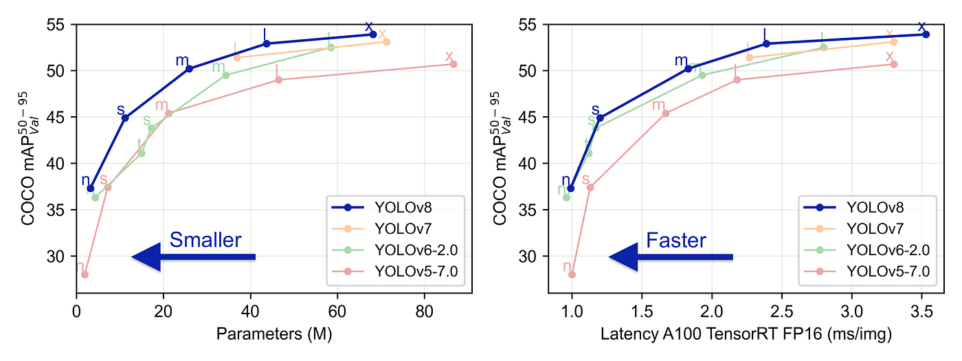
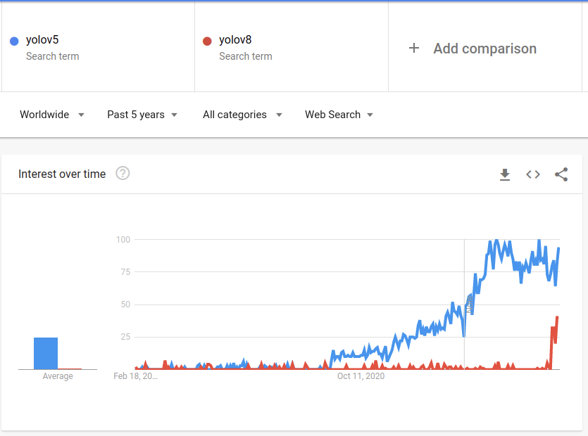
YOLOv8 was launched on January 10th, 2023. And as of this moment, this is the state-of-the-art model for classification, detection, and segmentation tasks in the computer vision world. The model outperforms all known models both in terms of accuracy and execution time.

The ultralytics team did a really good job in making this model easier to use compared to all the previous YOLO models — you don’t even have to clone the git repository anymore!

Creating the Image Dataset

In this post, I created a very simple example of all you need to do to train YOLOv8 on your data, specifically for a segmentation task. The dataset is small and “easy to learn” for the model, on purpose, so that we would be able to get satisfying results after training for only a few seconds on a simple CPU.

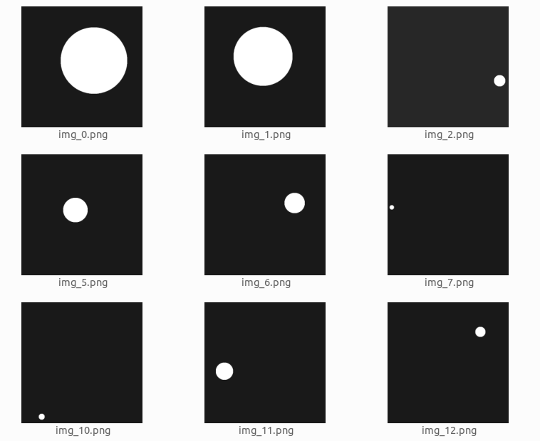
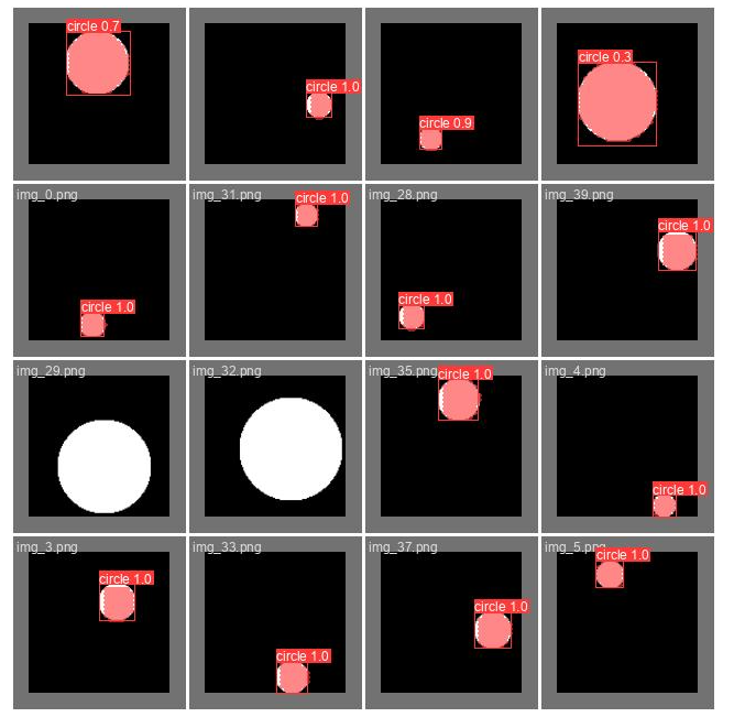
We will create a dataset of white circles with a black background. The circles will be of varying sizes. We will train a model that segments the circles inside the image.

This is what the dataset looks like:

The dataset was generated using the following code:

import numpy as np

from PIL import Image

from skimage import draw

import random

from pathlib import Path



def create_image(path, img_size, min_radius):

    path.parent.mkdir( parents=True, exist_ok=True )

    

    arr = np.zeros((img_size, img_size)).astype(np.uint8)

    center_x = random.randint(min_radius, (img_size-min_radius))

    center_y = random.randint(min_radius, (img_size-min_radius))

    max_radius = min(center_x, center_y, img_size - center_x, img_size - center_y)

    radius = random.randint(min_radius, max_radius)



    row_indxs, column_idxs = draw.ellipse(center_x, center_y, radius, radius, shape=arr.shape)

    

    arr[row_indxs, column_idxs] = 255



    im = Image.fromarray(arr)

    im.save(path)



def create_images(data_root_path, train_num, val_num, test_num, img_size=640, min_radius=10):

    data_root_path = Path(data_root_path)

    

    for i in range(train_num):

        create_image(data_root_path / 'train' / 'images' / f'img_{i}.png', img_size, min_radius)

        

    for i in range(val_num):

        create_image(data_root_path / 'val' / 'images' / f'img_{i}.png', img_size, min_radius)

        

    for i in range(test_num):

        create_image(data_root_path / 'test' / 'images' / f'img_{i}.png', img_size, min_radius)



create_images('datasets', train_num=120, val_num=40, test_num=40, img_size=120, min_radius=10)

Creating Labels

Now that we have an image dataset, we need to create labels for the images. Usually, we would need to do some manual work for this, but because the dataset we created is very simple, it is pretty easy to create code that generates labels for us:

from rasterio import features



def create_label(image_path, label_path):

    arr = np.asarray(Image.open(image_path))



    # There may be a better way to do it, but this is what I have found so far

    cords = list(features.shapes(arr, mask=(arr >0)))[0][0]['coordinates'][0]

    label_line = '0 ' + ' '.join([f'{int(cord[0])/arr.shape[0]} {int(cord[1])/arr.shape[1]}' for cord in cords])



    label_path.parent.mkdir( parents=True, exist_ok=True )

    with label_path.open('w') as f:

        f.write(label_line)



for images_dir_path in [Path(f'datasets/{x}/images') for x in ['train', 'val', 'test']]:

    for img_path in images_dir_path.iterdir():

        label_path = img_path.parent.parent / 'labels' / f'{img_path.stem}.txt'

        label_line = create_label(img_path, label_path)

Here is an example of a label file content:

0 0.0767 0.08433 0.1417 0.08433 0.1417 0.0917 0.15843 0.0917 0.15843 0.1 0.1766 0.1 0.1766 0.10844 0.175 0.10844 0.175 0.1177 0.18432 0.1177 0.18432 0.14333 0.1918 0.14333 0.1918 0.20844 0.18432 0.20844 0.18432 0.225 0.175 0.225 0.175 0.24334 0.1766 0.24334 0.1766 0.2417 0.15843 0.2417 0.15843 0.25 0.1417 0.25 0.1417 0.25846 0.0767 0.25846 0.0767 0.25 0.05 0.25 0.05 0.2417 0.04174 0.2417 0.04174 0.24334 0.04333 0.24334 0.04333 0.225 0.025 0.225 0.025 0.20844 0.01766 0.20844 0.01766 0.14333 0.025 0.14333 0.025 0.1177 0.04333 0.1177 0.04333 0.10844 0.04174 0.10844 0.04174 0.1 0.05 0.1 0.05 0.0917 0.0767 0.0917 0.0767 0.08433

The label corresponds to this image:

The label content is only a single text line. We have only one object (circle) in each image, and each object is represented by a line in the file. If you have more than one object in each image, you should create a line for each labeled object.

The first 0 represents the class type of the label. Because we have only one class type (a circle) we always have 0. If you have more than one class in your data, you should map each class to a number ( 0, 1, 2…) and use this number in the label file.

All the other numbers represent the coordinates of the bounding polygon of the labeled object. The format is <x1 y1 x2 y2 x3 y3…> and the coordinates are relative to the size of the image —you should normalize the coordinates to a 1x1 image size. For example, if there is a point (15, 75) and the image size is 120x120 the normalized point is (15/120, 75/120) = (0.125, 0.625).

It is always confusing when dealing with image libraries to get the correct directionality of the coordinates. So to make this clear, for YOLO, the X coordinate goes from left to right, and the Y coordinate goes from top to bottom.

The YAML Configuration

We have the images and the labels. Now we need to create a YAML file with the dataset configuration:

yaml_content = f'''

train: train/images

val: val/images

test: test/images



names: ['circle']

    '''

    

with Path('data.yaml').open('w') as f:

    f.write(yaml_content)

Pay attention that if you have more object class types, you need to add them here in the names array, in the same order you ordered them in the label files. The first is 0, the second is 1, etc…

Dataset File Structure

Let's see the file structure we created, using the Linux tree command:

tree .

data.yaml

datasets/

├── test

│   ├── images

│   │   ├── img_0.png

│   │   ├── img_1.png

│   │   ├── img_2.png

│   │   ├── ...

│   └── labels

│       ├── img_0.txt

│       ├── img_1.txt

│       ├── img_2.txt

│       ├── ...

├── train

│   ├── images

│   │   ├── img_0.png

│   │   ├── img_1.png

│   │   ├── img_2.png

│   │   ├── ...

│   └── labels

│       ├── img_0.txt

│       ├── img_1.txt

│       ├── img_2.txt

│       ├── ...

|── val

|   ├── images

│   │   ├── img_0.png

│   │   ├── img_1.png

│   │   ├── img_2.png

│   │   ├── ...

|   └── labels

│       ├── img_0.txt

│       ├── img_1.txt

│       ├── img_2.txt

│       ├── ...

Training The Model

Now that we have the images and the labels, we can start training the model. So first of all let's install the package:

pip install ultralytics==8.0.38

The ultralytics library changes pretty fast and sometimes breaks the API, so I prefer to stick with one version. The below code depends on version 8.0.38 (the newest version at the time I write those words). If you upgrade to a newer version, maybe you will need to do some code adaptations to make it work.

And start the training:

from ultralytics import YOLO



model = YOLO("yolov8n-seg.pt")



results = model.train(

        batch=8,

        device="cpu",

        data="data.yaml",

        epochs=7,

        imgsz=120,

    )

For the simplicity of this post, I use the nano model (yolov8n-seg), I train it only on the CPU, with only 7 epochs. The training took just a few seconds on my laptop.

For more information about the parameters that can be used to train the model, you can check this.

Understanding the Results

After the training is done you will see a line, similar to this, at the end of the output:

Results saved to runs/segment/train60

Let’s take a look at some of the results found here:

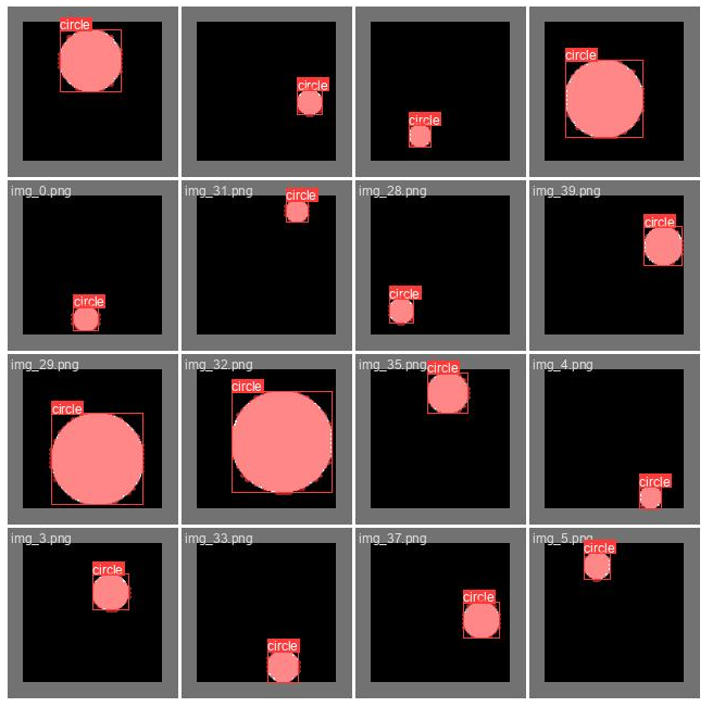
Validation labels

from IPython.display import Image as show_image

show_image(filename="runs/segment/train60/val_batch0_labels.jpg")

Here we can see the ground truth labels on part of the validation set. This should be almost perfectly aligned. In case you see those labels do not cover the objects well, it is highly likely that your labeling is incorrect.

Predicted validation labels

show_image(filename="runs/segment/train60/val_batch0_pred.jpg")

Here we can see the predictions the trained model did on part of the validation set (the same part we saw above). This can give you a feeling of how well the model performs. Pay attention that in order to create this image a confidence threshold should be chosen, the threshold used here is 0.5, which is not always the optimal one (we will discuss it later).

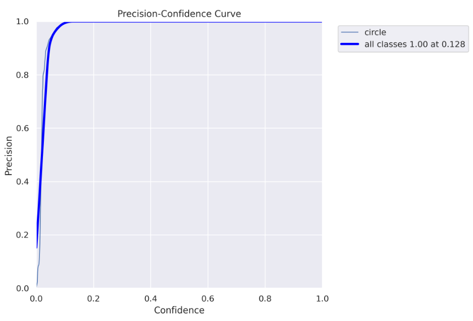
Precision curve

To understand this and the next charts you need to be familiar with precision and recall concepts. Here is a good explanation of how they work.

show_image(filename="runs/segment/train60/MaskP_curve.png")

Every detected object by the model has some confidence, usually, if it is important to you to be as sure as possible when declaring “this is a circle” you will use only high confidence values (high confidence threshold). Off course, it comes with a tradeoff- you can miss some “circles”. On the other hand, if you want to “catch” as many “circles” as you can with a tradeoff that some of them are not really “circles” you would use both low and high confidence values (low confidence threshold).

The above chart (and the chart below) helps you decide which confidence threshold to use. In our case, we can see that for a threshold higher than 0.128, we get 100% precision, which means all objects are correctly predicted.

Pay attention that because we actually doing a segmentation task, there is another important threshold we need to worry about — IoU ( intersection over union), if you are not familiar with it, you can read about it here. For this chart, an IoU of 0.5 is used.

Recall curve

show_image(filename="runs/segment/train60/MaskR_curve.png")

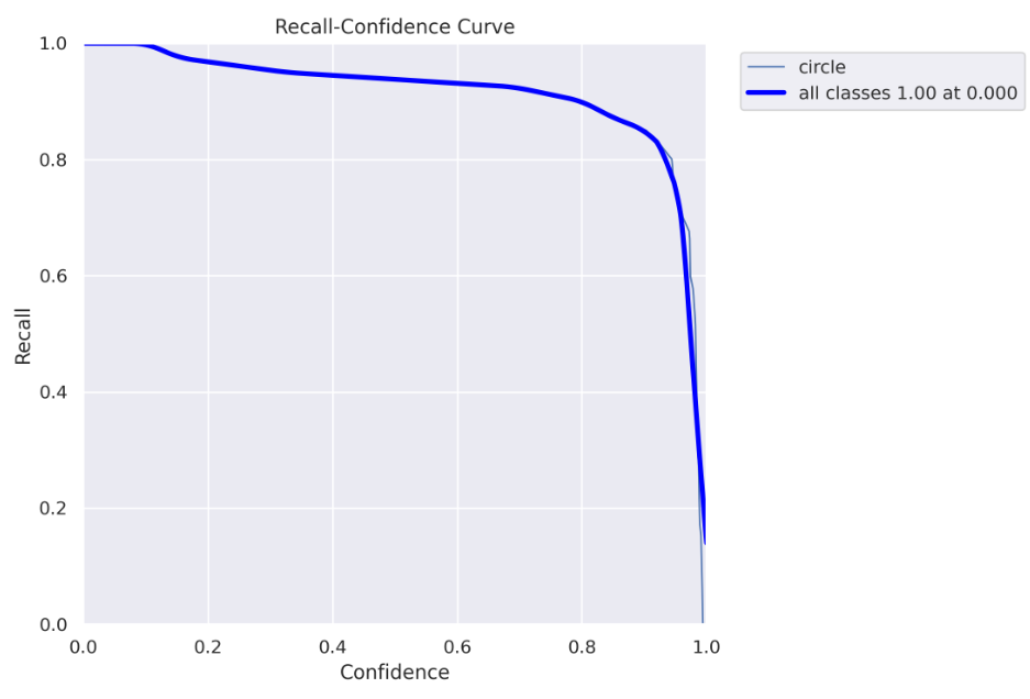
Here you can see the recall chart, as the confidence threshold values go up, the recall goes down. Which means you “catch” fewer “circles”.

Here you can see why using the 0.5 confidence threshold, in this case, is a bad idea. For a 0.5 threshold, you get about 90% recall. However, in the precision curve, we saw that for a threshold above 0.128, we get 100% precision, so we don’t need to get to 0.5, we can safely use a 0.128 threshold and get both 100% precision and almost 100% recall :)

Precision-Recall curve

Here is a good explanation of the precision-recall curve

show_image(filename="runs/segment/train60/MaskPR_curve.png")

We can see here clearly the conclusion we made before, for this model, we can get to almost 100% precision and 100% recall.

The disadvantage of this chart is that we can’t see what threshold we should use, this is why we still need the charts above.

Loss over time

show_image(filename="runs/segment/train60/results.png")

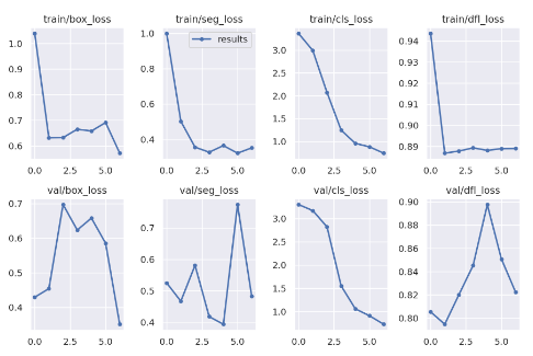
Here you can see how the different losses change during the training, and how they behave on the validation set after each epoch.

There is a lot to say about the losses, and conclusions you can make from those charts, however, it is out of the scope of this post. I just wanted to state that you can find it here :)

Using the trained model

Another thing that can be found in the result directory is the model itself. Here’s how to use the model on new images:

my_model = YOLO('runs/segment/train60/weights/best.pt')

results = list(my_model('datasets/test/images/img_5.png', conf=0.128))

result = results[0]

The results list may have multiple values, one for each detected object. Because in this example we have only one object in each image, we take the first list item.

You can see I passed here the best confidence threshold value we found before (0.128).

There are two ways to get the actual placement of the detected object in the image. Choosing the right method depends on what you intend to do with the results. I will show both ways.

result.masks.segments

[array([[    0.10156,     0.34375],

        [    0.09375,     0.35156],

        [    0.09375,     0.35937],

        [   0.078125,       0.375],

        [   0.070312,       0.375],

        [     0.0625,     0.38281],

        [    0.38281,     0.71094],

        [    0.39062,     0.71094],

        [    0.39844,     0.70312],

        [    0.39844,     0.69531],

        [    0.41406,     0.67969],

        [    0.42187,     0.67969],

        [    0.44531,     0.46875],

        [    0.42969,     0.45312],

        [    0.42969,     0.41406],

        [    0.42187,     0.40625],

        [    0.41406,     0.40625],

        [    0.39844,     0.39062],

        [    0.39844,     0.38281],

        [    0.39062,       0.375],

        [    0.38281,       0.375],

        [    0.35156,     0.34375]], dtype=float32)]

This returns the bounding polygon of the object, similar to the format we passed the labeled data.

And the second way:

result.masks.masks

tensor([[[0., 0., 0.,  ..., 0., 0., 0.],

         [0., 0., 0.,  ..., 0., 0., 0.],

         [0., 0., 0.,  ..., 0., 0., 0.],

         ...,

         [0., 0., 0.,  ..., 0., 0., 0.],

         [0., 0., 0.,  ..., 0., 0., 0.],

         [0., 0., 0.,  ..., 0., 0., 0.]]])

This returns a tensor with a shape (1, 128, 128) that represents all the pixels in the image. Pixels that are part of the object receive 1 and background pixels receive 0.

Let’s see what the mask looks like:

import torchvision.transforms as T

T.ToPILImage()(result.masks.masks).show()

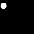
This was the original image:

Not perfect, but good enough for many applications, and the IoU is definitely higher than 0.5.

In conclusion, the new ultralytics library is much easier to work with compared to the previous Yolo versions, especially for the segmentation task, which is now a first-class citizen. You can find Yolov5 also as part of the ultralytics new package, so if you don’t want to use the new Yolo version, which is still kind of new and experimental, you can just use the well-known yolov5:

There were some topics I didn’t cover, like the different loss functions used for the model, the architecture changes that were made to create the yolov8, and more. Feel free to comment on this post if you want more information about those topics. If there will be interest, I will maybe write another post about it.

Thanks for taking the time to read this and I hope it helped you understand the Yolov8 model training process.

Supported Dataset Formats

Ultralytics YOLO format(Yolo数据格式)

The dataset label format used for training YOLO segmentation models is as follows:

1. One text file per image(每张图片对应一个txt文件): Each image in the dataset has a corresponding text file with the same name as the image file and the ".txt" extension.
2. One row per object(一个目标一行): Each row in the text file corresponds to one object instance in the image.
3. Object information per row: Each row contains the following information about the object instance:
   • Object class index: An integer representing the class of the object (e.g., 0 for person, 1 for car, etc.).
   • Object bounding coordinates: The bounding coordinates around the mask area, normalized to be between 0 and 1.

The format for a single row in the segmentation dataset file is as follows:

<class-index> <x1> <y1> <x2> <y2> ... <xn> <yn>

In this format, <class-index> is the index of the class for the object, and <x1> <y1> <x2> <y2> ... <xn> <yn> are the bounding coordinates of the object's segmentation mask. The coordinates are separated by spaces.

Here is an example of the YOLO dataset format for a single image with two objects made up of a 3-point segment and a 5-point segment.

0 0.681 0.485 0.670 0.487 0.676 0.4871 0.504 0.000 0.501 0.004 0.498 0.004 0.493 0.010 0.492 0.0104

Dataset YAML format

The Ultralytics framework uses a YAML file format to define the dataset and model configuration for training Detection Models. Here is an example of the YAML format used for defining a detection dataset:

# Train/val/test sets as 1) dir: path/to/imgs, 2) file: path/to/imgs.txt, or 3) list: [path/to/imgs1, path/to/imgs2, ..]path: ../datasets/coco8-seg # dataset root dir (absolute or relative; if relative, it's relative to default datasets_dir)train: images/train # train images (relative to 'path') 4 imagesval: images/val # val images (relative to 'path') 4 imagestest: # test images (optional)# Classes (80 COCO classes)names:    0: person    1: bicycle    2: car    # ...    77: teddy bear    78: hair drier    79: toothbrush

The train and val fields specify the paths to the directories containing the training and validation images, respectively.

names is a dictionary of class names. The order of the names should match the order of the object class indices in the YOLO dataset files.

Usage

# Start training from a pretrained *.pt modelyolo segment train data=coco8-seg.yaml model=yolo11n-seg.pt epochs=100 imgsz=640

Supported Datasets

Supported Datasets

• COCO: A comprehensive dataset for object detection, segmentation, and captioning, featuring over 200K labeled images across a wide range of categories.
• COCO8-seg: A compact, 8-image subset of COCO designed for quick testing of segmentation model training, ideal for CI checks and workflow validation in the ultralytics repository.
• COCO128-seg: A smaller dataset for instance segmentation tasks, containing a subset of 128 COCO images with segmentation annotations.
• Carparts-seg: A specialized dataset focused on the segmentation of car parts, ideal for automotive applications. It includes a variety of vehicles with detailed annotations of individual car components.
• Crack-seg: A dataset tailored for the segmentation of cracks in various surfaces. Essential for infrastructure maintenance and quality control, it provides detailed imagery for training models to identify structural weaknesses.
• Package-seg: A dataset dedicated to the segmentation of different types of packaging materials and shapes. It's particularly useful for logistics and warehouse automation, aiding in the development of systems for package handling and sorting.

Adding your own dataset

If you have your own dataset and would like to use it for training segmentation models with Ultralytics YOLO format, ensure that it follows the format specified above under "Ultralytics YOLO format". Convert your annotations to the required format and specify the paths, number of classes, and class names in the YAML configuration file.

Port or Convert Label Formats

COCO Dataset Format to YOLO Format

You can easily convert labels from the popular COCO dataset format to the YOLO format using the following code snippet:

from ultralytics.data.converter import convert_cococonvert_coco(labels_dir="path/to/coco/annotations/", use_segments=True)

This conversion tool can be used to convert the COCO dataset or any dataset in the COCO format to the Ultralytics YOLO format.

Remember to double-check if the dataset you want to use is compatible with your model and follows the necessary format conventions. Properly formatted datasets are crucial for training successful object detection models.

Auto-Annotation

Auto-annotation is an essential feature that allows you to generate a segmentation dataset using a pre-trained detection model. It enables you to quickly and accurately annotate a large number of images without the need for manual labeling, saving time and effort.

Generate Segmentation Dataset Using a Detection Model

To auto-annotate your dataset using the Ultralytics framework, you can use the auto_annotate function as shown below:

from ultralytics.data.annotator import auto_annotateauto_annotate(data="path/to/images", det_model="yolo11x.pt", sam_model="sam_b.pt")

The auto_annotate function takes the path to your images, along with optional arguments for specifying the pre-trained detection models i.e. YOLO11, YOLOv8 or other models and segmentation models i.e, SAM, SAM2 or MobileSAM, the device to run the models on, and the output directory for saving the annotated results.

By leveraging the power of pre-trained models, auto-annotation can significantly reduce the time and effort required for creating high-quality segmentation datasets. This feature is particularly useful for researchers and developers working with large image collections, as it allows them to focus on model development and evaluation rather than manual annotation.

FAQ

What dataset formats does Ultralytics YOLO support for instance segmentation?

Ultralytics YOLO supports several dataset formats for instance segmentation, with the primary format being its own Ultralytics YOLO format. Each image in your dataset needs a corresponding text file with object information segmented into multiple rows (one row per object), listing the class index and normalized bounding coordinates. For more detailed instructions on the YOLO dataset format, visit the Instance Segmentation Datasets Overview.

How can I convert COCO dataset annotations to the YOLO format?

Converting COCO format annotations to YOLO format is straightforward using Ultralytics tools. You can use the convert_coco function from the ultralytics.data.converter module:

from ultralytics.data.converter import convert_cococonvert_coco(labels_dir="path/to/coco/annotations/", use_segments=True)

This script converts your COCO dataset annotations to the required YOLO format, making it suitable for training your YOLO models. For more details, refer to Port or Convert Label Formats.

How do I prepare a YAML file for training Ultralytics YOLO models?

To prepare a YAML file for training YOLO models with Ultralytics, you need to define the dataset paths and class names. Here's an example YAML configuration:

path: ../datasets/coco8-seg # dataset root dirtrain: images/train # train images (relative to 'path')val: images/val # val images (relative to 'path')names:    0: person    1: bicycle    2: car    # ...

Ensure you update the paths and class names according to your dataset. For more information, check the Dataset YAML Format section.

What is the auto-annotation feature in Ultralytics YOLO?

Auto-annotation in Ultralytics YOLO allows you to generate segmentation annotations for your dataset using a pre-trained detection model. This significantly reduces the need for manual labeling. You can use the auto_annotate function as follows:

from ultralytics.data.annotator import auto_annotateauto_annotate(data="path/to/images", det_model="yolo11x.pt", sam_model="sam_b.pt")  # or sam_model="mobile_sam.pt"

This function automates the annotation process, making it faster and more efficient. For more details, explore the Auto-Annotate Reference.

Oriented Bounding Boxes Object Detection

Oriented object detection goes a step further than object detection and introduce an extra angle to locate objects more accurate in an image.

The output of an oriented object detector is a set of rotated bounding boxes that exactly enclose the objects in the image, along with class labels and confidence scores for each box. Object detection is a good choice when you need to identify objects of interest in a scene, but don't need to know exactly where the object is or its exact shape.

Watch: Object Detection using Ultralytics YOLO Oriented Bounding Boxes (YOLO-OBB)

Visual Samples

Ships Detection using OBB	Vehicle Detection using OBB

Models

YOLO11 pretrained OBB models are shown here, which are pretrained on the DOTAv1 dataset.

Models download automatically from the latest Ultralytics release on first use.

• mAP^test values are for single-model multiscale on DOTAv1 dataset.
  Reproduce by yolo val obb data=DOTAv1.yaml device=0 split=test and submit merged results to DOTA evaluation.
• Speed averaged over DOTAv1 val images using an Amazon EC2 P4d instance.
  Reproduce by yolo val obb data=DOTAv1.yaml batch=1 device=0|cpu

Train

Train YOLO11n-obb on the DOTA8 dataset for 100 epochs at image size 640. For a full list of available arguments see the Configuration page.

# Build a new model from YAML and start training from scratchyolo obb train data=dota8.yaml model=yolo11n-obb.yaml epochs=100 imgsz=640# Start training from a pretrained *.pt modelyolo obb train data=dota8.yaml model=yolo11n-obb.pt epochs=100 imgsz=640# Build a new model from YAML, transfer pretrained weights to it and start trainingyolo obb train data=dota8.yaml model=yolo11n-obb.yaml pretrained=yolo11n-obb.pt epochs=100 imgsz=640

Watch: How to Train Ultralytics YOLO-OBB (Oriented Bounding Boxes) Models on DOTA Dataset using Ultralytics HUB

Dataset format

OBB dataset format can be found in detail in the Dataset Guide.

Val

Validate trained YOLO11n-obb model accuracy on the DOTA8 dataset. No arguments are needed as the model retains its training data and arguments as model attributes.

yolo obb val model=yolo11n-obb.pt data=dota8.yaml  # val official modelyolo obb val model=path/to/best.pt data=path/to/data.yaml  # val custom model

Predict

Use a trained YOLO11n-obb model to run predictions on images.

yolo obb predict model=yolo11n-obb.pt source='https://ultralytics.com/images/boats.jpg'  # predict with official modelyolo obb predict model=path/to/best.pt source='https://ultralytics.com/images/boats.jpg'  # predict with custom model

Watch: How to Detect and Track Storage Tanks using Ultralytics YOLO-OBB | Oriented Bounding Boxes | DOTA

See full predict mode details in the Predict page.

Export

Export a YOLO11n-obb model to a different format like ONNX, CoreML, etc.

yolo export model=yolo11n-obb.pt format=onnx  # export official modelyolo export model=path/to/best.pt format=onnx  # export custom trained model

Available YOLO11-obb export formats are in the table below. You can export to any format using the format argument, i.e. format='onnx' or format='engine'. You can predict or validate directly on exported models, i.e. yolo predict model=yolo11n-obb.onnx. Usage examples are shown for your model after export completes.

See full export details in the Export page.

FAQ

What are Oriented Bounding Boxes (OBB) and how do they differ from regular bounding boxes?

Oriented Bounding Boxes (OBB) include an additional angle to enhance object localization accuracy in images. Unlike regular bounding boxes, which are axis-aligned rectangles, OBBs can rotate to fit the orientation of the object better. This is particularly useful for applications requiring precise object placement, such as aerial or satellite imagery (Dataset Guide).

How do I train a YOLO11n-obb model using a custom dataset?

To train a YOLO11n-obb model with a custom dataset, follow the example below using Python or CLI:

yolo obb train data=path/to/custom_dataset.yaml model=yolo11n-obb.pt epochs=100 imgsz=640

For more training arguments, check the Configuration section.

What datasets can I use for training YOLO11-OBB models?

YOLO11-OBB models are pretrained on datasets like DOTAv1 but you can use any dataset formatted for OBB. Detailed information on OBB dataset formats can be found in the Dataset Guide.

How can I export a YOLO11-OBB model to ONNX format?

Exporting a YOLO11-OBB model to ONNX format is straightforward using either Python or CLI:

yolo export model=yolo11n-obb.pt format=onnx

For more export formats and details, refer to the Export page.

How do I validate the accuracy of a YOLO11n-obb model?

To validate a YOLO11n-obb model, you can use Python or CLI commands as shown below:

yolo obb val model=yolo11n-obb.pt data=dota8.yaml

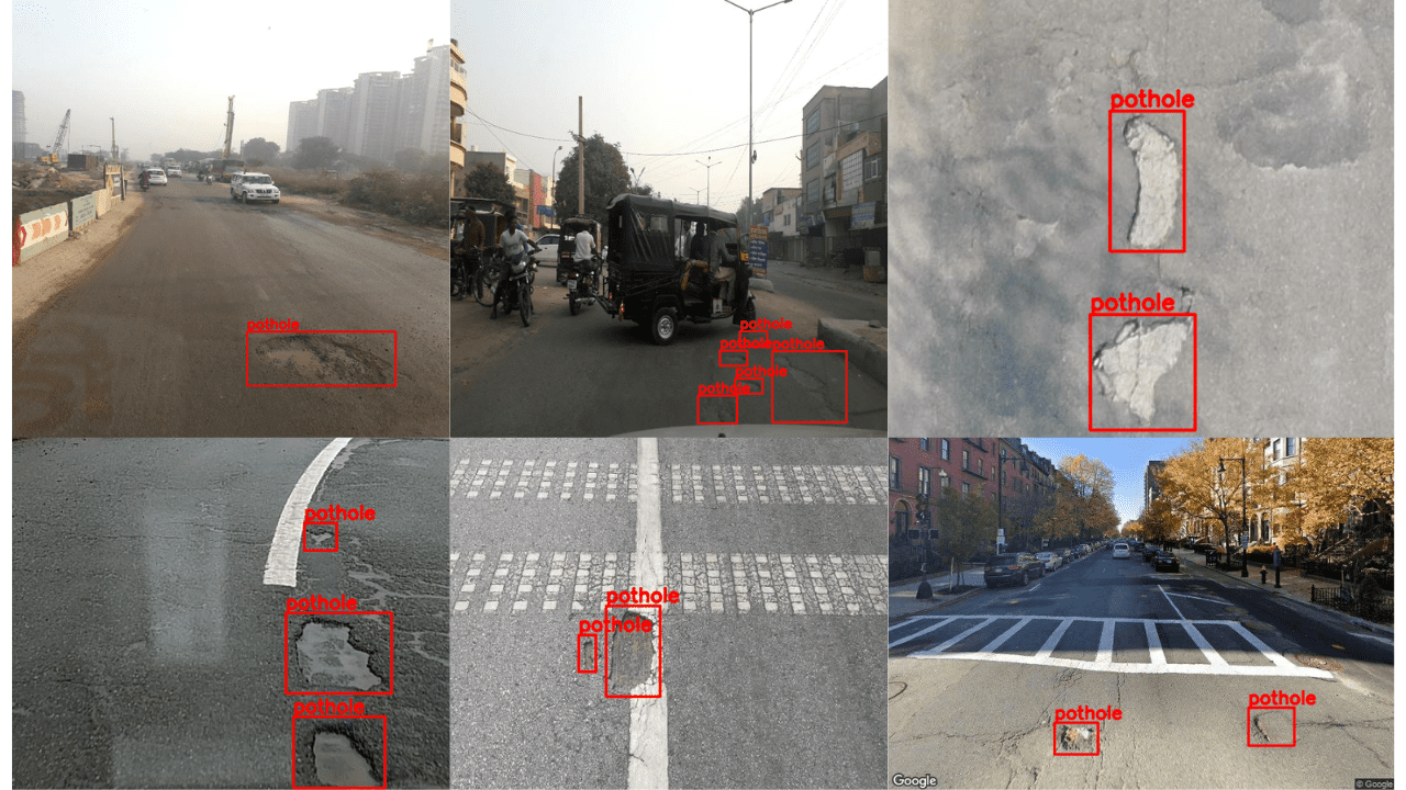
Ultralytics recently released the YOLOv8 family of object detection models. These models outperform the previous versions of YOLO models in both speed and accuracy on the COCO dataset. But what about the performance on custom datasets? To answer this, we will train YOLOv8 models on a custom dataset. Specifically, we will train it on a large scale pothole detection dataset.

While fine tuning object detection models, we need to consider a large number of hyperparameters into account. Training the YOLOv8 models is no exception, as the codebase provides numerous hyperparameters for tuning. Moreover, we will train the YOLOv8 on a custom pothole dataset which mainly contains small objects which can be difficult to detect. 

To get the best model, we need to conduct several training experiments and evaluate each. As such, we will train three different YOLOv8 models:

• YOLOv8n (Nano model)
• YOLOv8s (Small model)
• YOLOv8m (Medium model)

After training, we will also run inference on videos to check the real-world performance of these models. This will give us a better idea of the best model among the three.

In addition to these, you will also learn how to use ClearML for logging and monitoring YOLOv8 model training.

• The Pothole Detection Dataset to Train YOLOv8
• Setting Up YOLOv8 to Train on Custom Dataset
• Train YOLOv8 on the Custom Pothole Detection Dataset
• YOLO8 Nano Training on the Pothole Detection Dataset
• YOLO8 Small Training on the Pothole Detection Dataset
• YOLO8 Medium Training on the Pothole Detection Dataset
• YOLOv8n vs YOLOv8s vs YOLOv8m
• Inference using the Trained YOLOv8 Models
• Summary and Conclusion

YOLO Master Post –  Every Model Explained

Unlock the full story behind all the YOLO models’ evolutionary journey: Dive into our extensive pillar post, where we unravel the evolution from YOLOv1 to YOLO-NAS. This essential guide is packed with insights, comparisons, and a deeper understanding that you won’t find anywhere else.
Don’t miss out on this comprehensive resource, Mastering All Yolo Models for a richer, more informed perspective on the YOLO series.

Mastering All YOLO Models from YOLOv1 to YOLO-NAS: Papers Explained (2024)

The Pothole Detection Dataset to Train YOLOv8

We are using quite a large pothole dataset in this article which contains more than 7000 images collected from several sources.

To give a brief overview, the dataset includes images from:

• Roboflow pothole dataset
• Dataset from a research paper publication
• Images that have been sourced from YouTube videos and are manually annotated
• Images from the RDD2022 dataset

After going through several annotation corrections, the final dataset now contains:

• 6962 training images
• 271 validation images

Here are a few images from the dataset, along with the annotations.

It is very clear from the above image that training YOLOv8 on a custom pothole dataset is a very challenging task. The potholes can be of various sizes, ranging from small to large.

Download the Dataset

If you plan to execute the training commands on your local system, you can download the dataset by executing the following command.

Next, unzip it in the current directory.

Inside the directory, we are the dataset is contained in the train and valid folders. As with all other YOLO models, the labels are in the text files with normalized xcenter, ycenter, width, height.

The Pothole Dataset YAML File

For training, we need the dataset YAML to define the paths to the images and the class names.

Click here to download the source code to this post

According to the training commands, we will execute further in this article, this YAML file should be in the project root directory. We will name this file pothole_v8.yaml.

According to the above file, the pothole_dataset_v8 directory should be present in the current working directory.

Setting Up YOLOv8 to Train on Custom Dataset

To train YOLOv8 on a custom dataset, we need to install the ultralytics package. This provides the yolo Command Line Interface (CLI). One big advantage is that we do not need to clone the repository separately and install the requirements.

Note: Before moving further into the installation steps, please install CUDA and cuDNN if you want to execute the training steps in your system.
We can install the package using pip.

The above package will install all the dependencies, including Torchvision and PyTorch.

Setting Up ClearML

We do not want to be monitoring our deep learning experiments manually. So, we will use the ClearML integration, which Ultralytics YOLOv8 supports by default. We just need to install the package and initialize it using the API.

Next, we need to add the API key. But before that, we need to generate a key. Follow the steps to generate and add the key:

• Create a ClearML account.
• Go to Settings => Workspace and click on create new credentials

• Copy the information under the LOCAL PYTHON tab.
• Open the terminal and activate the environment in which CearML is installed. Type and execute clearml-init.
• This will prompt you to paste the above-copied information. That’s it; your ClearML credentials are added to the system.

From now on, any YOLOv8 training experiments that you run in this terminal will be logged into your ClearML dashboard.

Train YOLOv8 on the Custom Pothole Detection Dataset

In this section, we will conduct three experiments using three different YOLOv8 models. We will train the YOLOv8 Nano, Small, and Medium models on the dataset.

Hyperparameter Choices to Train YOLOv8 on Custom Dataset

Here are a few pointers explaining the hyperparameter choices that we make while training:

• We will train each model for 50 epochs. As a concept project, to get started, we will try to get the best possible results with limited training. As we have almost 7000 images, even 50 epochs will take quite some time to train and should give decent results.
• To have a fair comparison between the models, we will set the batch size to 8 in all the experiments,
• As the potholes can be quite small in some images, we will set the image size to 1280 resolution while training. Although this will increase the training time, we can expect better results compared to the default 640 image resolution training.

All the training experiments were carried out on a machine with 24 GB RTX 3090 GPU, Xeon E5-2697 processor, and 32 GB RAM.

As the pothole detection dataset is quite challenging, we will mostly focus on the mAP at 0.50 IoU (Intersection over Union).

Commands for Training YOLOv8 on Custom Dataset

We can either use the CLI or Python API to train the YOLOv8 models. Before moving on to the actual training phase, let’s check out the commands and the possible arguments we may need to deal with.

This is a sample training command using the Nano model.

Here are the explanations of all the command line arguments that we are using:

• task: Whether we want to detect, segment, or classify on the dataset of our choice.
• mode: Mode can either be train, val, or predict. As we are running training, it should be train.
• model: The model that we want to use. Here, we use the YOLOv8 Nano model pretrained on the COCO dataset.
• imgsz: The image size. The default resolution is 640.
• data: Path to the dataset YAML file.
• epochs: Number of epochs we want to train for.
• batch: The batch size for data loader. You may increase or decrease it according to your GPU memory availability.
• name: Name of the results directory for runs/detect.

You may also create a Python file (say train.py) and use the Ultralytics Python API to train the model. The following is an example of the same.

In the next section, we will move on to the actual training experiments and modify the command line arguments wherever necessary.

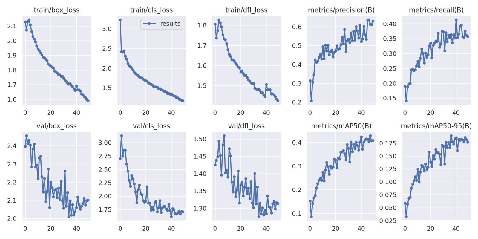
YOLO8 Nano Training on the Pothole Detection Dataset

Starting with the YOLO8 Nano model training, the smallest in the YOLOv8 family. This model has 3.2 million parameters and can run in real-time, even on a CPU.
You may execute the following command in the terminal to start the training. This is using the Yolo CLI.

Here are a few pointers regarding the training:

• We are training the model for 50 epochs, which will stay the same for all the models.
• As discussed earlier, we are training with a 1280 which is higher than the default 640.
• The batch size is 8.

The following code block shows the same training setup but using the Python API.

The training will take a few hours to complete depending on the hardware.

Following are the final plots saved to the local directory after the entire training completes.

We can also evaluate the best model using the following command.

We get the following result on the validation set.

The highest mAP (Mean Average Precision) at 0.50 IoU is 40.4 and at 0.50:0.95 IoU is 18.9. It may seem less but considering that it is a Nano model, it’s not that bad.

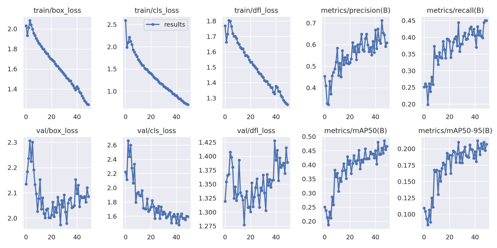
YOLO8 Small Training on the Pothole Detection Dataset

Now, let’s train the YOLOv8 Small model on the pothole dataset and check it’s performance.

As was in the previous case, we can also use the Python API to train the model.

We only need to change the model from yolov8n.pt to yolov8s.pt.

Using the YOLOv8 Small model, we reach almost an mAP of 50 at 0.50 IoU. Let’s run the evaluation command to check the actual value.

Here are the results.

The model reaches an mAP of 49. It is quite good for a small model. Mostly, the image size of 1280 is helping a lot in reaching such numbers.

YOLO8 Medium Training on the Pothole Detection Dataset

For the final experiment, we will train the YOLOv8 Medium model on the pothole dataset.

Following is the corresponding Python API code.

This time, we are passing the model as yolov5m.pt.

The YOLOv8 medium model also seems to reach an mAP of nearly 50. Let’s run the evaluation to get the actual numbers.

Interestingly, the YOLOv8 Medium model reaches an mAP of 48 within 50 epochs compared to the mAP of 49 using the small model.

YOLOv8n vs YOLOv8s vs YOLOv8m

As you may remember, we set up ClearML at the beginning of the article. All the training results were logged into the ClearML dashboard for each experiment.

Here is a graph from ClearML showing the comparison between each of the YOLOv8 models trained on the pothole dataset.

The above graph showing the mAP of all three models at 0.50 IoU is giving a much clearer picture. Apart from the YOLOv8 Nano model, the other two models are improving all the way through training. And we can train these two models for even longer to get better results.

Inference using the Trained YOLOv8 Models

Currently, we have three well performing models with us. For the next step of experiments, we will run inference and compare the results.

Note: The inference experiments were performed on a laptop with 6 GB GTX 1060 GPU, 8th generation i7 CPU, and 16 GB RAM.

Let’s run inference on a video using the trained YOLOv8 Nano model.

To run inference, we change the mode to predict and provide the path to the desired model weights. The source takes either path to a folder containing images and videos or the path to a single file. You may provide the path to a video file of your choice to run inference.

Remember to provide the same imgsz as we did while training to get the best results. As we have only one class, we use hide_labels=True to make the visualizations a bit cleaner.

Here are the results.

On the GTX 1060 GPU, the forward pass was running at almost 58 FPS which is pretty fast with a 1280 image resolution.

The results are fluctuating a bit, and also the model is only able to detect the potholes only when they are near.

Here is a comparison between all three on the same video to get a better idea of which model performs the best.

Interestingly, the medium model is detecting more potholes farther away in the first few frames, even though it had less mAP compared to the YOLOv8 Small model.

For reference, the YOLOv8 Small model runs at 35 FPS and the YOLOv8 Medium model runs at 14 FPS.

Here is another comparison between the YOLOv8 Medium and YOLOv8 Small models. 

The results look almost identical here due to their very close validation mAP. But in a few frames, the YOLOv8 Medium model seems to detect smaller potholes.

Most probably, with longer training, the YOLOv8 Medium model will surpass the YOLOv8 Small model. 

Summary and Conclusion

In this article, we had a detailed walkthrough to train the YOLOv8 models on a custom dataset. In the process, we also carried out a small real-world training experiment for pothole detection. 

The experiments revealed that training object detection models on small objects could be challenging even with sufficient samples. We could observe this as training for 50 epochs was insufficient, and the mAP graphs were still increasing. Also, with smaller objects, larger object detection models (YOLOv8 Medium vs Nano in this case) seem to perform better when carrying out detection on new images and videos.

Here is a quick summary of all the points that we covered:

• We started with the setting up of YOLOv8 and Ultralytics.
• Then we saw how to set up ClearML for logging.
• After preparing the dataset, we conducted three different YOLOv8 training experiments.
• Finally, we ran evaluation and inference to compare the three trained models.

If you extend this project, we would love to hear about your experience in the comment section.

References

• Ultralytics
• YOLOv8 Docs
• Dataset references:
  • Roboflow
  • ResearchGate research
  • RDD dataset