Automatic Addison 机器人入门学习
网站:
https://automaticaddison.com/tutorials/
网站:
https://automaticaddison.com/tutorials/
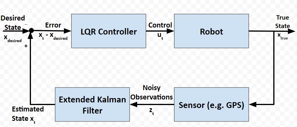
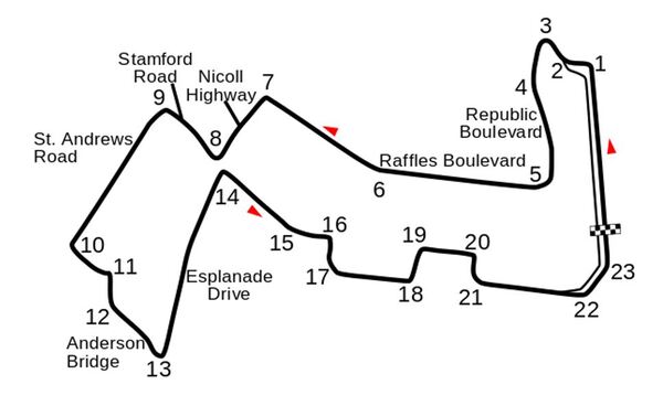
I recently built a project to combine the Extended Kalman Filter (for state estimation) and the Linear Quadratic Regulator (for control) to drive a simulated path-following race car (which is modeled as a point) around a track that is the same shape as the Formula 1 Singapore Grand Prix Marina Bay Street Circuit race track.
In a real-world application, it is common for a robot to use the Extended Kalman Filter to calculate near-optimal estimates of the state of a robotic system and to use LQR to generate the control values that move the robot from one state to the next.
Here is a block diagram of that process:
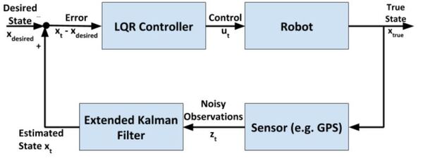
At each timestep:
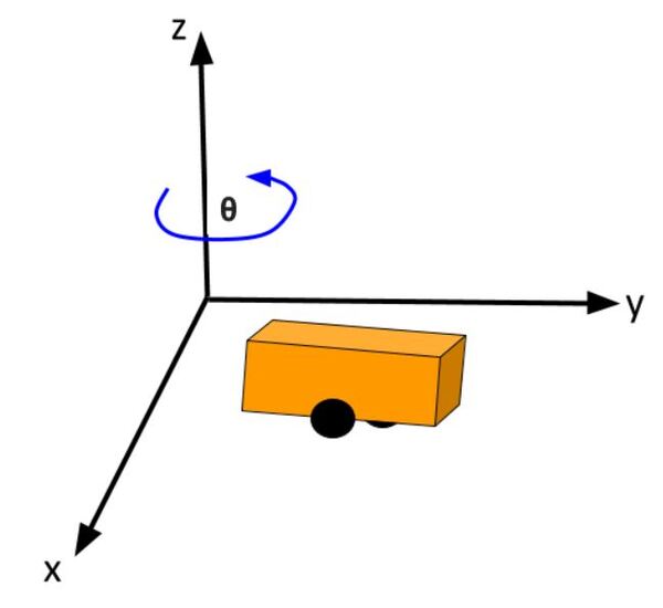
The kinematics of the system are modeled according to the following diagrams:
In my application, I assume there are sensors mounted on the race car that help it to localize itself in the x-y coordinate plane. These sensors measure the range (r) and bearing (b) from the race car to each landmark. Each landmark has a known x and y position.
The programs I developed were written in Python and use the same sequence of actions as indicated in the block diagram (in the first part of this post) in order to follow the race track (which is a list of waypoints).
You will need to put these five Python (3.7 or higher) programs into a single directory.
cubic_spine_planner.py
1
2
3
4
5
6
7
8
9
10
11
12
13
14
15
16
17
18
19
20
21
22
23
24
25
26
27
28
29
30
31
32
33
34
35
36
37
38
39
40
41
42
43
44
45
46
47
48
49
50
51
52
53
54
55
56
57
58
59
60
61
62
63
64
65
66
67
68
69
70
71
72
73
74
75
76
77
78
79
80
81
82
83
84
85
86
87
88
89
90
91
92
93
94
95
96
97
98
99
100
101
102
103
104
105
106
107
108
109
110
111
112
113
114
115
116
117
118
119
120
121
122
123
124
125
126
127
128
129
130
131
132
133
134
135
136
137
138
139
140
141
142
143
144
145
146
147
148
149
150
151
152
153
154
155
156
157
158
159
160
161
162
163
164
165
166
167
168
169
170
171
172
173
174
175
176
177
178
179
180
181
182
183
184
185
186
187
188
189
190
191
192
193
194
195
196
197
198
199
200
201
202
203
204
205
206
207
208
209
210
211
212
213
214
215
216
217
218
219
220
221
222
223
224
225
226
227
228
229
230
231
232
233
234
235
236
237
238
239
240
241
242
243
|
"""Cubic spline plannerProgram: cubic_spine_planner.pyAuthor: Atsushi Sakai(@Atsushi_twi)This program implements a cubic spline. For more information on cubic splines, check out this link:"""import mathimport numpy as npimport bisectclass Spline: """ Cubic Spline class """ def __init__(self, x, y): self.b, self.c, self.d, self.w = [], [], [], [] self.x = x self.y = y self.nx = len(x) # dimension of x h = np.diff(x) # calc coefficient c self.a = [iy for iy in y] # calc coefficient c A = self.__calc_A(h) B = self.__calc_B(h) self.c = np.linalg.solve(A, B) # print(self.c1) # calc spline coefficient b and d for i in range(self.nx - 1): self.d.append((self.c[i + 1] - self.c[i]) / (3.0 * h[i])) tb = (self.a[i + 1] - self.a[i]) / h[i] - h[i] * \ (self.c[i + 1] + 2.0 * self.c[i]) / 3.0 self.b.append(tb) def calc(self, t): """ Calc position if t is outside of the input x, return None """ if t < self.x[0]: return None elif t > self.x[-1]: return None i = self.__search_index(t) dx = t - self.x[i] result = self.a[i] + self.b[i] * dx + \ self.c[i] * dx ** 2.0 + self.d[i] * dx ** 3.0 return result def calcd(self, t): """ Calc first derivative if t is outside of the input x, return None """ if t < self.x[0]: return None elif t > self.x[-1]: return None i = self.__search_index(t) dx = t - self.x[i] result = self.b[i] + 2.0 * self.c[i] * dx + 3.0 * self.d[i] * dx ** 2.0 return result def calcdd(self, t): """ Calc second derivative """ if t < self.x[0]: return None elif t > self.x[-1]: return None i = self.__search_index(t) dx = t - self.x[i] result = 2.0 * self.c[i] + 6.0 * self.d[i] * dx return result def __search_index(self, x): """ search data segment index """ return bisect.bisect(self.x, x) - 1 def __calc_A(self, h): """ calc matrix A for spline coefficient c """ A = np.zeros((self.nx, self.nx)) A[0, 0] = 1.0 for i in range(self.nx - 1): if i != (self.nx - 2): A[i + 1, i + 1] = 2.0 * (h[i] + h[i + 1]) A[i + 1, i] = h[i] A[i, i + 1] = h[i] A[0, 1] = 0.0 A[self.nx - 1, self.nx - 2] = 0.0 A[self.nx - 1, self.nx - 1] = 1.0 # print(A) return A def __calc_B(self, h): """ calc matrix B for spline coefficient c """ B = np.zeros(self.nx) for i in range(self.nx - 2): B[i + 1] = 3.0 * (self.a[i + 2] - self.a[i + 1]) / \ h[i + 1] - 3.0 * (self.a[i + 1] - self.a[i]) / h[i] return Bclass Spline2D: """ 2D Cubic Spline class """ def __init__(self, x, y): self.s = self.__calc_s(x, y) self.sx = Spline(self.s, x) self.sy = Spline(self.s, y) def __calc_s(self, x, y): dx = np.diff(x) dy = np.diff(y) self.ds = [math.sqrt(idx ** 2 + idy ** 2) for (idx, idy) in zip(dx, dy)] s = [0] s.extend(np.cumsum(self.ds)) return s def calc_position(self, s): """ calc position """ x = self.sx.calc(s) y = self.sy.calc(s) return x, y def calc_curvature(self, s): """ calc curvature """ dx = self.sx.calcd(s) ddx = self.sx.calcdd(s) dy = self.sy.calcd(s) ddy = self.sy.calcdd(s) k = (ddy * dx - ddx * dy) / ((dx ** 2 + dy ** 2)**(3 / 2)) return k def calc_yaw(self, s): """ calc yaw """ dx = self.sx.calcd(s) dy = self.sy.calcd(s) yaw = math.atan2(dy, dx) return yawdef calc_spline_course(x, y, ds=0.1): sp = Spline2D(x, y) s = list(np.arange(0, sp.s[-1], ds)) rx, ry, ryaw, rk = [], [], [], [] for i_s in s: ix, iy = sp.calc_position(i_s) rx.append(ix) ry.append(iy) ryaw.append(sp.calc_yaw(i_s)) rk.append(sp.calc_curvature(i_s)) return rx, ry, ryaw, rk, sdef main(): print("Spline 2D test") import matplotlib.pyplot as plt x = [-2.5, 0.0, 2.5, 5.0, 7.5, 3.0, -1.0] y = [0.7, -6, 5, 6.5, 0.0, 5.0, -2.0] ds = 0.1 # [m] distance of each intepolated points sp = Spline2D(x, y) s = np.arange(0, sp.s[-1], ds) rx, ry, ryaw, rk = [], [], [], [] for i_s in s: ix, iy = sp.calc_position(i_s) rx.append(ix) ry.append(iy) ryaw.append(sp.calc_yaw(i_s)) rk.append(sp.calc_curvature(i_s)) flg, ax = plt.subplots(1) plt.plot(x, y, "xb", label="input") plt.plot(rx, ry, "-r", label="spline") plt.grid(True) plt.axis("equal") plt.xlabel("x[m]") plt.ylabel("y[m]") plt.legend() flg, ax = plt.subplots(1) plt.plot(s, [math.degrees(iyaw) for iyaw in ryaw], "-r", label="yaw") plt.grid(True) plt.legend() plt.xlabel("line length[m]") plt.ylabel("yaw angle[deg]") flg, ax = plt.subplots(1) plt.plot(s, rk, "-r", label="curvature") plt.grid(True) plt.legend() plt.xlabel("line length[m]") plt.ylabel("curvature [1/m]") plt.show()if __name__ == '__main__': main() |
kinematics.py
1
2
3
4
5
6
7
8
9
10
11
12
13
14
15
16
17
18
19
20
21
22
23
24
25
26
27
28
29
30
31
32
33
34
35
36
37
38
39
40
41
42
43
44
45
46
47
48
49
50
51
52
53
54
55
56
57
58
59
60
61
62
63
64
65
66
67
68
69
70
71
72
73
74
75
76
77
78
79
80
81
82
83
84
85
86
87
88
89
90
91
92
93
94
95
96
97
98
99
100
101
102
103
104
105
106
107
108
109
110
111
112
113
114
115
116
117
118
119
120
121
122
123
124
125
126
127
128
129
130
131
132
133
134
135
136
137
138
139
140
141
142
143
144
145
146
147
148
149
150
151
152
153
154
155
156
157
158
159
160
161
162
163
164
165
166
167
168
169
170
171
172
173
174
175
176
177
178
179
180
181
182
183
184
185
186
187
188
189
190
191
192
193
194
195
196
197
198
199
200
201
202
203
204
205
206
207
208
209
210
211
212
213
214
215
216
217
218
219
220
221
222
223
224
225
226
227
228
229
230
231
232
233
234
235
236
237
238
239
240
241
242
243
244
245
246
247
248
249
250
251
252
253
254
255
256
257
258
259
260
261
262
263
264
265
266
267
268
269
270
271
272
273
274
275
276
277
278
279
280
281
282
283
284
285
286
287
288
289
290
291
292
293
294
295
296
297
298
299
300
301
302
303
|
""" Implementation of the two-wheeled differential drive robot car and its controller.Our goal in using LQR is to find the optimal control inputs: [linear velocity of the car, angular velocity of the car] We want to both minimize the error between the current state and a desired state, while minimizing actuator effort (e.g. wheel rotation rate). These are competing objectives because a large u (i.e. wheel rotation rates) expends a lot ofactuator energy but can drive the state error to 0 really fast.LQR helps us balance these competing objectives.If a system is linear, LQR gives the optimal control inputs that takes a system's state to 0, where the state is"current state - desired state".Implemented by Addison Sears-CollinsDate: December 10, 2020"""# Import required librariesimport numpy as npimport scipy.linalg as laclass DifferentialDrive(object): """ Implementation of Differential Drive kinematics. This represents a two-wheeled vehicle defined by the following states state = [x,y,theta] where theta is the yaw angle and accepts the following control inputs input = [linear velocity of the car, angular velocity of the car] """ def __init__(self): """ Initializes the class """ # Covariance matrix representing action noise # (i.e. noise on the control inputs) self.V = None def get_state_size(self): """ The state is (X, Y, THETA) in global coordinates, so the state size is 3. """ return 3 def get_input_size(self): """ The control input is ([linear velocity of the car, angular velocity of the car]), so the input size is 2. """ return 2 def get_V(self): """ This function provides the covariance matrix V which describes the noise that can be applied to the forward kinematics. Feel free to experiment with different levels of noise. Output :return: V: input cost matrix (3 x 3 matrix) """ # The np.eye function returns a 2D array with ones on the diagonal # and zeros elsewhere. if self.V is None: self.V = np.eye(3) self.V[0,0] = 0.01 self.V[1,1] = 0.01 self.V[2,2] = 0.1 return 1e-5*self.V def forward(self,x0,u,v,dt=0.1): """ Computes the forward kinematics for the system. Input :param x0: The starting state (position) of the system (units:[m,m,rad]) np.array with shape (3,) -> (X, Y, THETA) :param u: The control input to the system 2x1 NumPy Array given the control input vector is [linear velocity of the car, angular velocity of the car] [meters per second, radians per second] :param v: The noise applied to the system (units:[m, m, rad]) ->np.array with shape (3,) :param dt: Change in time (units: [s]) Output :return: x1: The new state of the system (X, Y, THETA) """ u0 = u # If there is no noise applied to the system if v is None: v = 0 # Starting state of the vehicle X = x0[0] Y = x0[1] THETA = x0[2] # Control input u_linvel = u0[0] u_angvel = u0[1] # Velocity in the x and y direction in m/s x_dot = u_linvel * np.cos(THETA) y_dot = u_linvel * np.sin(THETA) # The new state of the system x1 = np.empty(3) # Calculate the new state of the system # Noise is added like in slide 34 in Lecture 7 x1[0] = x0[0] + x_dot * dt + v[0] # X x1[1] = x0[1] + y_dot * dt + v[1] # Y x1[2] = x0[2] + u_angvel * dt + v[2] # THETA return x1 def linearize(self, x, dt=0.1): """ Creates a linearized version of the dynamics of the differential drive robotic system (i.e. a robotic car where each wheel is controlled separately. The system's forward kinematics are nonlinear due to the sines and cosines, so we need to linearize it by taking the Jacobian of the forward kinematics equations with respect to the control inputs. Our goal is to have a discrete time system of the following form: x_t+1 = Ax_t + Bu_t where: Input :param x: The state of the system (units:[m,m,rad]) -> np.array with shape (3,) -> (X, Y, THETA) -> X_system = [x1, x2, x3] :param dt: The change in time from time step t to time step t+1 Output :return: A: Matrix A is a 3x3 matrix (because there are 3 states) that describes how the state of the system changes from t to t+1 when no control command is executed. Typically, a robotic car only drives when the wheels are turning. Therefore, in this case, A is the identity matrix. :return: B: Matrix B is a 3 x 2 matrix (because there are 3 states and 2 control inputs) that describes how the state (X, Y, and THETA) changes from t to t + 1 due to the control command u. Matrix B is found by taking the The Jacobian of the three forward kinematics equations (for X, Y, THETA) with respect to u (3 x 2 matrix) """ THETA = x[2] ####### A Matrix ####### # A matrix is the identity matrix A = np.array([[1.0, 0, 0], [ 0, 1.0, 0], [ 0, 0, 1.0]]) ####### B Matrix ####### B = np.array([[np.cos(THETA)*dt, 0], [np.sin(THETA)*dt, 0], [0, dt]]) return A, Bdef dLQR(F,Q,R,x,xf,dt=0.1): """ Discrete-time linear quadratic regulator for a non-linear system. Compute the optimal control given a nonlinear system, cost matrices, a current state, and a final state. Compute the control variables that minimize the cumulative cost. Solve for P using the dynamic programming method. Assume that Qf = Q Input: :param F: The dynamics class object (has forward and linearize functions implemented) :param Q: The state cost matrix Q -> np.array with shape (3,3) :param R: The input cost matrix R -> np.array with shape (2,2) :param x: The current state of the system x -> np.array with shape (3,) :param xf: The desired state of the system xf -> np.array with shape (3,) :param dt: The size of the timestep -> float Output :return: u_t_star: Optimal action u for the current state [linear velocity of the car, angular velocity of the car] [meters per second, radians per second] """ # We want the system to stabilize at xf, # so we let x - xf be the state. # Actual state - desired state x_error = x - xf # Calculate the A and B matrices A, B = F.linearize(x, dt) # Solutions to discrete LQR problems are obtained using dynamic # programming. # The optimal solution is obtained recursively, starting at the last # time step and working backwards. N = 50 # Create a list of N + 1 elements P = [None] * (N + 1) # Assume Qf = Q Qf = Q # 1. LQR via Dynamic Programming P[N] = Qf # 2. For t = N, ..., 1 for t in range(N, 0, -1): # Discrete-time Algebraic Riccati equation to calculate the optimal # state cost matrix P[t-1] = Q + A.T @ P[t] @ A - (A.T @ P[t] @ B) @ la.pinv( R + B.T @ P[t] @ B) @ (B.T @ P[t] @ A) # Create a list of N elements K = [None] * N u = [None] * N # 3 and 4. For t = 0, ..., N - 1 for t in range(N): # Calculate the optimal feedback gain K_t K[t] = -la.pinv(R + B.T @ P[t+1] @ B) @ B.T @ P[t+1] @ A for t in range(N): # Calculate the optimal control input u[t] = K[t] @ x_error # Optimal control input is u_t_star u_t_star = u[N-1] # Return the optimal control inputs return u_t_stardef get_R(): """ This function provides the R matrix to the lqr_ekf_control simulator. Returns the input cost matrix R. Experiment with different gains. This matrix penalizes actuator effort (i.e. rotation of the motors on the wheels). The R matrix has the same number of rows as are actuator states [linear velocity of the car, angular velocity of the car] [meters per second, radians per second] This matrix often has positive values along the diagonal. We can target actuator states where we want low actuator effort by making the corresponding value of R large. Output :return: R: Input cost matrix """ R = np.array([[0.01, 0], # Penalization for linear velocity effort [0, 0.01]]) # Penalization for angular velocity effort return Rdef get_Q(): """ This function provides the Q matrix to the lqr_ekf_control simulator. Returns the state cost matrix Q. Experiment with different gains to see their effect on the vehicle's behavior. Q helps us weight the relative importance of each state in the state vector (X, Y, THETA). Q is a square matrix that has the same number of rows as there are states. Q penalizes bad performance. Q has positive values along the diagonal and zeros elsewhere. Q enables us to target states where we want low error by making the corresponding value of Q large. We can start with the identity matrix and tweak the values through trial and error. Output :return: Q: State cost matrix (3x3 matrix because the state vector is (X, Y, THETA)) """ Q = np.array([[0.4, 0, 0], # Penalize X position error (global coordinates) [0, 0.4, 0], # Penalize Y position error (global coordinates) [0, 0, 0.4]])# Penalize heading error (global coordinates) return Q |
lqr_ekf_control.py
1
2
3
4
5
6
7
8
9
10
11
12
13
14
15
16
17
18
19
20
21
22
23
24
25
26
27
28
29
30
31
32
33
34
35
36
37
38
39
40
41
42
43
44
45
46
47
48
49
50
51
52
53
54
55
56
57
58
59
60
61
62
63
64
65
66
67
68
69
70
71
72
73
74
75
76
77
78
79
80
81
82
83
84
85
86
87
88
89
90
91
92
93
94
95
96
97
98
99
100
101
102
103
104
105
106
107
108
109
110
111
112
113
114
115
116
117
118
119
120
121
122
123
124
125
126
127
128
129
130
131
132
133
134
135
136
137
138
139
140
141
142
143
144
145
146
147
148
149
150
151
152
153
154
155
156
157
158
|
"""A robot will follow a racetrack using an LQR controller and EKF (with landmarks)to estimate the state (i.e. x position, y position, yaw angle) at each timestep####################Adapted from code authored by Atsushi Sakai (@Atsushi_twi)"""# Import important librariesimport numpy as npimport mathimport matplotlib.pyplot as pltfrom kinematics import *from sensors import *from utils import *from time import sleepshow_animation = Truedef closed_loop_prediction(desired_traj, landmarks): ## Simulation Parameters T = desired_traj.shape[0] # Maximum simulation time goal_dis = 0.1 # How close we need to get to the goal goal = desired_traj[-1,:] # Coordinates of the goal dt = 0.1 # Timestep interval time = 0.0 # Starting time ## Initial States state = np.array([8.3,0.69,0]) # Initial state of the car state_est = state.copy() sigma = 0.1*np.ones(3) # State covariance matrix ## Get the Cost-to-go and input cost matrices for LQR Q = get_Q() # Defined in kinematics.py R = get_R() # Defined in kinematics.py ## Initialize the Car and the Car's landmark sensor DiffDrive = DifferentialDrive() LandSens = LandmarkDetector(landmarks) # Process noise and sensor measurement noise V = DiffDrive.get_V() W = LandSens.get_W() ## Create objects for storing states and estimated state t = [time] traj = np.array([state]) traj_est = np.array([state_est]) ind = 0 while T >= time: ## Point to track ind = int(np.floor(time)) goal_i = desired_traj[ind,:] ## Generate noise # v = process noise, w = measurement noise v = np.random.multivariate_normal(np.zeros(V.shape[0]),V) w = np.random.multivariate_normal(np.zeros(W.shape[0]),W) ## Generate optimal control commands u_lqr = dLQR(DiffDrive,Q,R,state_est,goal_i[0:3],dt) ## Move forwad in time state = DiffDrive.forward(state,u_lqr,v,dt) # Take a sensor measurement for the new state y = LandSens.measure(state,w) # Update the estimate of the state using the EKF state_est, sigma = EKF(DiffDrive,LandSens,y,state_est,sigma,u_lqr,dt) # Increment time time = time + dt # Store the trajectory and estimated trajectory t.append(time) traj = np.concatenate((traj,[state]),axis=0) traj_est = np.concatenate((traj_est,[state_est]),axis=0) # Check to see if the robot reached goal if np.linalg.norm(state[0:2]-goal[0:2]) <= goal_dis: print("Goal reached") break ## Plot the vehicles trajectory if time % 1 < 0.1 and show_animation: plt.cla() plt.plot(desired_traj[:,0], desired_traj[:,1], "-r", label="course") plt.plot(traj[:,0], traj[:,1], "ob", label="trajectory") plt.plot(traj_est[:,0], traj_est[:,1], "sk", label="estimated trajectory") plt.plot(goal_i[0], goal_i[1], "xg", label="target") plt.axis("equal") plt.grid(True) plt.title("SINGAPORE GRAND PRIX\n" + "speed[m/s]:" + str( round(np.mean(u_lqr), 2)) + ",target index:" + str(ind)) plt.pause(0.0001) #input() return t, trajdef main(): # Countdown to start print("\n*** SINGAPORE GRAND PRIX ***\n") print("Start your engines!") print("3.0") sleep(1.0) print("2.0") sleep(1.0) print("1.0\n") sleep(1.0) print("LQR + EKF steering control tracking start!!") # Create the track waypoints ax = [8.3,8.0, 7.2, 6.5, 6.2, 6.5, 1.5,-2.0,-3.5,-5.0,-7.9, -6.7,-6.7,-5.2,-3.2,-1.2, 0.0, 0.2, 2.5, 2.8, 4.4, 4.5, 7.8, 8.5, 8.3] ay = [0.7,4.3, 4.5, 5.2, 4.0, 0.7, 1.3, 3.3, 1.5, 3.0,-1.0, -2.0,-3.0,-4.5, 1.1,-0.7,-1.0,-2.0,-2.2,-1.2,-1.5,-2.4,-2.7,-1.7,-0.1] # These landmarks help the mobile robot localize itself landmarks = [[4,3], [8,2], [-1,-4]] # Compute the desired trajectory desired_traj = compute_traj(ax,ay) t, traj = closed_loop_prediction(desired_traj,landmarks) # Display the trajectory that the mobile robot executed if show_animation: plt.close() flg, _ = plt.subplots(1) plt.plot(ax, ay, "xb", label="input") plt.plot(desired_traj[:,0], desired_traj[:,1], "-r", label="spline") plt.plot(traj[:,0], traj[:,1], "-g", label="tracking") plt.grid(True) plt.axis("equal") plt.xlabel("x[m]") plt.ylabel("y[m]") plt.legend() plt.show()if __name__ == '__main__': main() |
sensors.py
1
2
3
4
5
6
7
8
9
10
11
12
13
14
15
16
17
18
19
20
21
22
23
24
25
26
27
28
29
30
31
32
33
34
35
36
37
38
39
40
41
42
43
44
45
46
47
48
49
50
51
52
53
54
55
56
57
58
59
60
61
62
63
64
65
66
67
68
69
70
71
72
73
74
75
76
77
78
79
80
81
82
83
84
85
86
87
88
89
90
91
92
93
94
95
96
97
98
99
100
101
102
103
104
105
106
107
108
109
110
111
112
113
114
115
116
117
118
119
120
121
122
123
124
125
126
127
128
129
130
131
132
133
134
135
136
137
138
139
140
141
142
143
144
145
146
147
148
149
150
151
152
153
154
155
156
157
158
159
160
161
162
163
164
165
166
167
168
169
170
171
172
173
174
175
176
177
178
179
180
181
182
183
184
185
186
187
188
189
190
191
192
193
194
195
196
197
198
199
200
201
202
203
204
205
206
207
208
209
210
211
212
213
214
215
216
217
218
219
220
221
222
223
224
225
226
227
228
229
230
231
232
233
234
235
236
237
238
239
240
241
242
243
244
245
246
247
248
249
250
251
252
253
254
255
256
257
258
259
260
|
"""Extended Kalman Filter implementation using landmarks to localizeImplemented by Addison Sears-CollinsDate: December 10, 2020"""import numpy as npimport scipy.linalg as laimport mathclass LandmarkDetector(object): """ This class represents the sensor mounted on the robot that is used to to detect the location of landmarks in the environment. """ def __init__(self,landmark_list): """ Calculates the sensor measurements for the landmark sensor Input :param landmark_list: 2D list of landmarks [L1,L2,L3,...,LN], where each row is a 2D landmark defined by Li =[l_i_x,l_i_y] which corresponds to its x position and y position in the global coordinate frame. """ # Store the x and y position of each landmark in the world self.landmarks = np.array(landmark_list) # Record the total number of landmarks self.N_landmarks = self.landmarks.shape[0] # Variable that represents landmark sensor noise (i.e. error) self.W = None def get_W(self): """ This function provides the covariance matrix W which describes the noise that can be applied to the sensor measurements. Feel free to experiment with different levels of noise. Output :return: W: measurement noise matrix (4x4 matrix given two landmarks) In this implementation there are two landmarks. Each landmark has an x location and y location, so there are 4 individual sensor measurements. """ # In the EKF code, we will condense this 4x4 matrix so that it is a 4x1 # landmark sensor measurement noise vector (i.e. [x1 noise, y1 noise, x2 # noise, y2 noise] if self.W is None: self.W = 0.0095*np.eye(2*self.N_landmarks) return self.W def measure(self,x,w=None): """ Computes the landmark sensor measurements for the system. This will be a list of range (i.e. distance) and relative angles between the robot and a set of landmarks defined with [x,y] positions. Input :param x: The state [x_t,y_t,theta_t] of the system -> np.array with shape (3,). x is a 3x1 vector :param w: The noise (assumed Gaussian) applied to the measurement -> np.array with shape (2 * N_Landmarks,) w is a 4x1 vector Output :return: y: The resulting observation vector (4x1 in this implementation because there are 2 landmarks). The resulting measurement is y = [h1_range_1,h1_angle_1, h2_range_2, h2_angle_2] """ # Create the observation vector y = np.zeros(shape=(2*self.N_landmarks,)) # Initialize state variables x_t = x[0] y_t = x[1] THETA_t = x[2] # Fill in the observation model y for i in range(0, self.N_landmarks): # Set the x and y position for landmark i x_l_i = self.landmarks[i][0] y_l_i = self.landmarks[i][1] # Set the noise value w_r = w[i*2] w_b = w[i*2+1] # Calculate the range (distance from robot to the landmark) and # bearing angle to the landmark range_i = math.sqrt(((x_t - x_l_i)**2) + ((y_t - y_l_i)**2)) + w_r angle_i = math.atan2(y_t - y_l_i,x_t - x_l_i) - THETA_t + w_b # Populate the predicted sensor observation vector y[i*2] = range_i y[i*2+1] = angle_i return y def jacobian(self,x): """ Computes the first order jacobian around the state x Input :param x: The starting state (position) of the system -> np.array with shape (3,) Output :return: H: The resulting Jacobian matrix H for the sensor. The number of rows is equal to two times the number of landmarks H. 2 rows (for the range (distance) and bearing to landmark measurement) x 3 columns for the number of states (X, Y, THETA). In other words, the number of rows is equal to the total number of individual sensor measurements. Since we have 2 landmarks, H will be a 4x3 matrix (2 * N_Landmarks x Number of states) """ # Create the Jacobian matrix H # For example, the first two rows of the Jacobian matrix H pertain to # the first landmark: # dh_range/dx_t dh_range/dy_t dh_range/dtheta_t # dh_bearing/dx_t dh_bearing/dy_t dh_bearing/dtheta_t # Note that 'bearing' and 'angle' are synonymous in this program. H = np.zeros(shape=(2 * self.N_landmarks, 3)) # Extract the state X_t = x[0] Y_t = x[1] THETA_t = x[2] # Fill in H, the Jacobian matrix with the partial derivatives of the # observation (measurement) model h # Partial derivatives were calculated using an online partial derivatives # calculator. # atan2 derivatives are listed here https://en.wikipedia.org/wiki/Atan2 for i in range(0, self.N_landmarks): # Set the x and y position for landmark i x_l_i = self.landmarks[i][0] y_l_i = self.landmarks[i][1] dh_range_dx_t = (X_t-x_l_i) / math.sqrt((X_t-x_l_i)**2 + (Y_t-y_l_i)**2) H[i*2][0] = dh_range_dx_t dh_range_dy_t = (Y_t-y_l_i) / math.sqrt((X_t-x_l_i)**2 + (Y_t-y_l_i)**2) H[i*2][1] = dh_range_dy_t dh_range_dtheta_t = 0 H[i*2][2] = dh_range_dtheta_t dh_bearing_dx_t = -(Y_t-y_l_i) / ((X_t-x_l_i)**2 + (Y_t-y_l_i)**2) H[i*2+1][0] = dh_bearing_dx_t dh_bearing_dy_t = (X_t-x_l_i) / ((X_t-x_l_i)**2 + (Y_t-y_l_i)**2) H[i*2+1][1] = dh_bearing_dy_t dh_bearing_dtheta_t = -1.0 H[i*2+1][2] = dh_bearing_dtheta_t return Hdef EKF(DiffDrive,Sensor,y,x_hat,sigma,u,dt,V=None,W=None): """ Some of these matrices will be non-square or singular. Utilize the pseudo-inverse function la.pinv instead of inv to avoid these errors. Input :param DiffDrive: The DifferentialDrive object defined in kinematics.py :param Sensor: The Landmark Sensor object defined in this class :param y: The observation vector (4x1 in this implementation because there are 2 landmarks). The measurement is y = [h1_range_1,h1_angle_1, h2_range_2, h2_angle_2] :param x_hat: The starting estimate of the state at time t -> np.array with shape (3,) (X_t, Y_t, THETA_t) :param sigma: The state covariance matrix at time t -> np.array with shape (3,1) initially, then 3x3 :param u: The input to the system at time t -> np.array with shape (2,1) These are the control inputs to the system. [left wheel rotational velocity, right wheel rotational velocity] :param dt: timestep size delta t :param V: The state noise covariance matrix -> np.array with shape (3,3) :param W: The measurment noise covariance matrix -> np.array with shape (2*N_Landmarks,2*N_Landmarks) 4x4 matrix Output :return: x_hat_2: The estimate of the state at time t+1 [X_t+1, Y_t+1, THETA_t+1] :return: sigma_est: The new covariance matrix at time t+1 (3x3 matrix) """ V = DiffDrive.get_V() # 3x3 matrix for the state noise W = Sensor.get_W() # 4x4 matrix for the measurement noise ## Generate noise # v = process noise, w = measurement noise v = np.random.multivariate_normal(np.zeros(V.shape[0]),V) # 3x1 vector w = np.random.multivariate_normal(np.zeros(W.shape[0]),W) # 4x1 vector ##### Prediction Step ##### # Predict the state estimate based on the previous state and the # control input # x_predicted is a 3x1 vector (X_t+1, Y_t+1, THETA_t+1) x_predicted = DiffDrive.forward(x_hat,u,v,dt) # Calculate the A and B matrices A, B = DiffDrive.linearize(x=x_hat) # Predict the covariance estimate based on the # previous covariance and some noise # A and V are 3x3 matrices sigma_3by3 = None if (sigma.size == 3): sigma_3by3 = sigma * np.eye(3) else: sigma_3by3 = sigma sigma_new = A @ sigma_3by3 @ A.T + V ##### Correction Step ##### # Get H, the 4x3 Jacobian matrix for the sensor H = Sensor.jacobian(x_hat) # Calculate the observation model # y_predicted is a 4x1 vector y_predicted = Sensor.measure(x_predicted, w) # Measurement residual (delta_y is a 4x1 vector) delta_y = y - y_predicted # Residual covariance # 4x3 @ 3x3 @ 3x4 -> 4x4 matrix S = H @ sigma_new @ H.T + W # Compute the Kalman gain # The Kalman gain indicates how certain you are about # the observations with respect to the motion # 3x3 @ 3x4 @ 4x4 -> 3x4 K = sigma_new @ H.T @ la.pinv(S) # Update the state estimate # 3x1 + (3x4 @ 4x1 -> 3x1) x_hat_2 = x_predicted + (K @ delta_y) # Update the covariance estimate # 3x3 - (3x4 @ 4x3) @ 3x3 sigma_est = sigma_new - (K @ H @ sigma_new) return x_hat_2 , sigma_est |
utils.py
1
2
3
4
5
6
7
8
9
10
11
12
13
14
15
16
17
18
19
20
21
22
23
24
25
26
27
28
29
30
31
32
33
34
35
36
37
38
39
40
41
42
43
44
45
46
47
48
49
50
51
52
53
54
55
56
57
58
59
60
61
62
63
64
65
66
67
68
69
70
71
72
73
|
"""Program: utils.pyThis program helps calculate the waypoints along the racetrackthat the robot needs to follow.Modified from code developed by Atsushi Sakai"""import numpy as npimport mathimport cubic_spline_plannerdef pi_2_pi(angle): return (angle + math.pi) % (2*math.pi) - math.pidef compute_traj(ax,ay): cx, cy, cyaw, ck, s = cubic_spline_planner.calc_spline_course( ax, ay, ds=0.1) target_speed = 1 # simulation parameter km/h -> m/s sp = calc_speed_profile(cx, cy, cyaw, target_speed) desired_traj = np.array([cx,cy,cyaw,sp]).T return desired_trajdef calc_nearest_index(state, traj): cx = traj[:,0] cy = traj[:,1] cyaw = traj[:,2] dx = [state[0] - icx for icx in cx] dy = [state[1] - icy for icy in cy] d = [idx ** 2 + idy ** 2 for (idx, idy) in zip(dx, dy)] mind = min(d) ind = d.index(mind) mind = math.sqrt(mind) dxl = cx[ind] - state[0] dyl = cy[ind] - state[1] angle = pi_2_pi(cyaw[ind] - math.atan2(dyl, dxl)) if angle < 0: mind *= -1 return ind, minddef calc_speed_profile(cx, cy, cyaw, target_speed): speed_profile = [target_speed] * len(cx) direction = 1.0 # Set stop point for i in range(len(cx) - 1): dyaw = abs(cyaw[i + 1] - cyaw[i]) switch = math.pi / 4.0 <= dyaw < math.pi / 2.0 if switch: direction *= -1 if direction != 1.0: speed_profile[i] = - target_speed else: speed_profile[i] = target_speed if switch: speed_profile[i] = 0.0 speed_profile[-1] = 0.0 return speed_profile |
To run the code, navigate to the directory and run the lqr_ekf_control.py program. I’m using Anaconda to run my Python programs, so I’ll type:
python lqr_ekf_control.py
Keep building!
In this tutorial, we will learn about the Linear Quadratic Regulator (LQR). At the end, I’ll show you my example implementation of LQR in Python.
To get started, let’s take a look at what LQR is all about. Since LQR is an optimal feedback control technique, let’s start with the definition of optimal feedback control and then build our way up to LQR.
Table of Contents
Here are a couple of real-world examples where you might find LQR control:
Consider these two real world examples:
How do you accomplish both of these tasks?
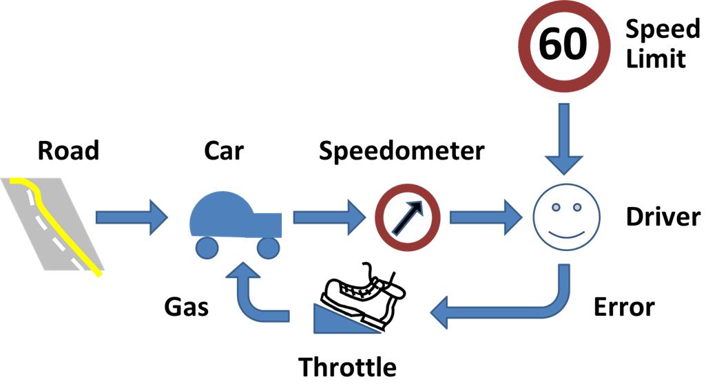
Both the robot and the drone need to have a feedback control algorithm running inside them.
The control algorithm’s job will be to output control signals (e.g. velocity of the wheels on the robot car, propeller speed, etc.) that reduce the error between the actual state (e.g. current position of the robot car or altitude for the drone) and the desired state.
The sensors on the robot car/drone need to read the state of the system and feed that information back to the controller.
The controller compares the actual state (i.e. the sensor information) with the desired state and then generates the best possible (i.e. optimal) control signals (often known as “system input”) that will reduce or eliminate that error.
In Example 1, the desired state is the (x,y) coordinate or GPS position along a predetermined path. At each timestep, you want the control algorithm to generate velocity commands for your robot that minimize the error between your current actual state (i.e. position) and the desired position (i.e. on top of the predetermined path).
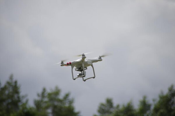
In Example 2, with the drone, you want to minimize the error between your desired altitude of the drone and the actual altitude of the drone.
Here is how all that looks in a picture:
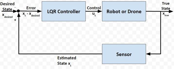
Your robot car and drone go through a continuous process of sensing the state of the system and then generating the best possible control commands to minimize the difference between the desired state xdesired and actual state xt.
The goal at each timestep (as the robot car drives along the path or the drone hovers in the air) is to use sensor feedback to drive the state error towards 0, where:
State error = xt – xdesired
Let’s revisit our examples from the previous section.
Suppose in Example 2, a strong wind from a thunderstorm began to blow the drone downward, causing it to fall way below the desired altitude.
To correct its altitude, the drone could:
Both Action 1 and 2 have pros and cons.
Action 1
Action 2
How can we write a smart controller that balances both objectives? We want the system to both:
This, my friends, is where the Linear Quadratic Regulator (LQR) comes to the rescue.
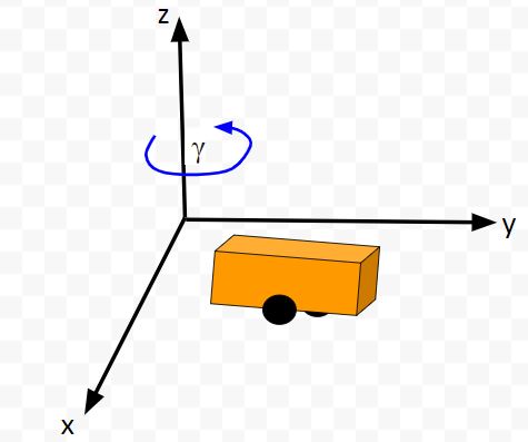
LQR solves a common problem when we’re trying to optimally control a robotic system. Going back to our robot car example, let’s draw its diagram. Here is our real world robot:
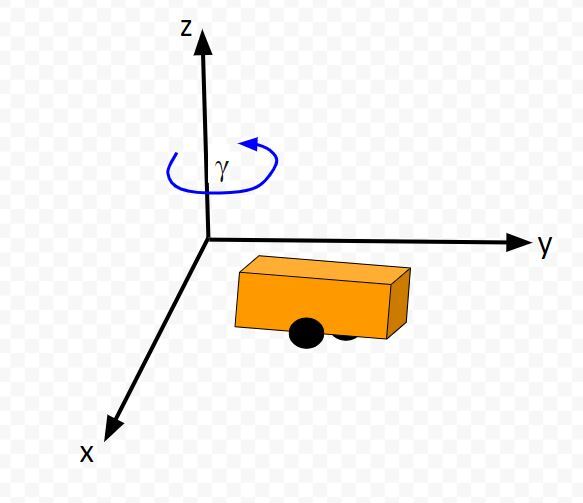
Let’s model this robot in a 3D diagram with coordinate axes x, y, and z:
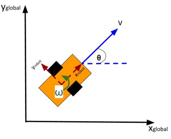
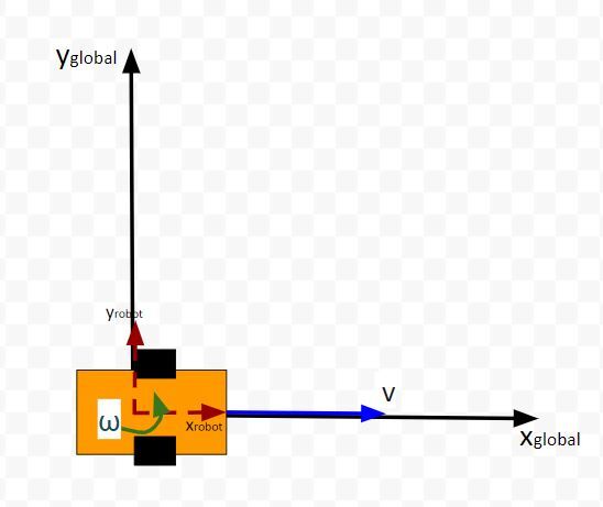
Here is the bird’s-eye view in 2D form:
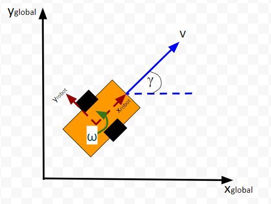
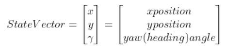
Suppose the robot car’s state at time t (position, orientation) is represented by vector xt (e.g. where xt = [xglobal, yglobal, orientation (yaw angle)].
A state space model for this robotic system might look like the following:
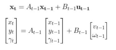
where
(If that equation above doesn’t make a lot of sense, please check out the tutorial in the Prerequisites of this article where I dive into it in detail)
We want to choose control inputs ut-1….such that
Both of these are competing objectives. A large u can drive the state error down really fast. A small u means the state error will remain really large. LQR was designed to solve this problem.
The purpose of LQR is to compute the optimal control inputs ut-1 (i.e. velocity of the wheels of a robotic car, motors for propellers of a drone) given:
that minimize the cumulative “cost.”
LQR is all about the cost function. It does some fancy math to come up with a function (this Wikipedia page shows the function) that expresses a “cost” (you could also substitute the word “penalty”) that is a function of both state error and actuator effort.
LQR’s goal is to minimize the “cost” of the state error, while minimizing the “cost” of actuator effort.
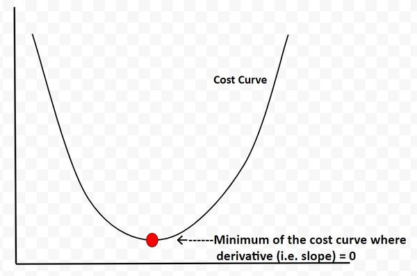
LQR determines the point along the cost curve where the “cost function” is minimized…thereby balancing both objectives of keeping state error and actuator effort minimized.
The cost curve below is for illustration purposes only. I’m using it just to explain this concept. In reality, the cost curve does not look like this. I’m using this graphic to convey to you the idea that LQR is all about finding the optimal control commands (i.e. linear velocity, angular velocity in the case of our robot car example) at which the actuator-effort state-error cost function is at a minimum. And from calculus, we know that the minimum of this cost function occurs at the point where the derivative (i.e. slope) is equal to 0.
We use some fancy math (I’ll get into this later) to find out what this point is.
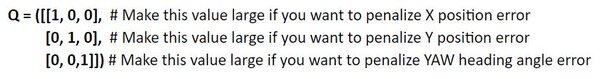
Q is called the state cost matrix. Q helps us weigh the relative importance of each state in the state vector (i.e. [x error,y error,yaw angle error]).
Q is a square matrix that has the same number of rows and columns as there are states.
Q penalizes bad performance (e.g. penalizes large differences between where you want the robot to be vs. where it actually is in the world)
Q has positive values along the diagonal and zeros elsewhere.
Q enables us to target states where we want low error by making the corresponding value of Q large.
I typically start out with the identity matrix and then tweak the values through trial and error. In a 3-state system, such as with our two-wheeled robot car, Q would be the following 3×3 matrix:
Similarly, R is the input cost matrix. This matrix penalizes actuator effort (i.e. rotation of the motors on the wheels).
The R matrix has the same number of rows as are control inputs and the same number of columns as are control inputs.
For example, imagine if we had a two-wheeled car with two control inputs, one for the linear velocity v and one for the angular velocity ω.
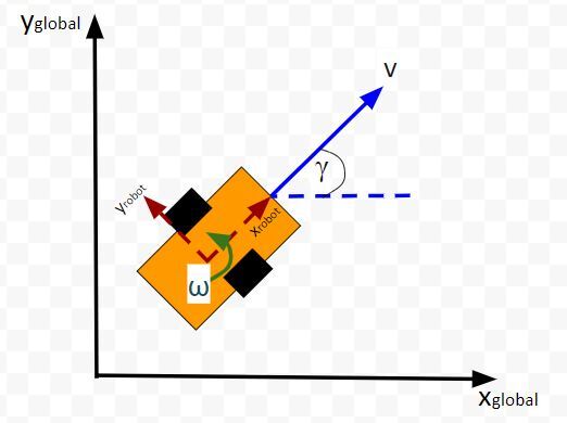
The control input vector ut-1 would be [linear velocity v in meters per second, angular velocity ω in radians per second].
The input cost matrix often has positive values along the diagonal. We can use this matrix to target actuator states where we want low actuator effort by making the corresponding value of R large.
A lot of people start with the identity matrix, but I’ll start out with some low numbers. You want to tweak the values through trial and error.
In a case where we have two control inputs into a robotic system, here would be my starting 2×2 R matrix:

LQR uses a technique called dynamic programming. You don’t need to worry what that means.
At each timestep t as the robot or drone moves in the world, the optimal control input is calculated using a series of for loops (where we run each for loop ~N times) that spit out the u (i.e. control inputs) that corresponds to the minimal overall cost.
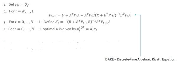
Here is the pseudocode for LQR. Hang tight. Go through this slowly. There is a lot of mathematical notation thrown around, and I want you to leave this tutorial with a solid understanding of LQR.
Let’s walk through this together. The pseudocode is in bold italics, and my comments are in plain text. You see below that the LQR function accepts 7 parameters.
LQR(Actual State x, Desired State xf, Q, R, A, B, dt):
x_error = Actual State x – Desired State xf
Initialize N = ##
I typically set N to some arbitrary integer like 50. Solutions to LQR problems are obtained recursively, starting at the last time step, and working backwards in time to the first time step.
In other words, the for loops (we’ll get to these in a second) need to go through lots of iterations (50 in this case) to reach a stable value for P (we’ll cover P in the next step).
Set P = [Empty list of N + 1 elements]
Let P[N] = Q
For i = N, …, 1
P[i-1] = Q + ATP[i]A – (ATP[i]B)(R + BTP[i]B)-1(BTP[i]A)
This ugly equation above is called the Discrete-time Algebraic Riccati equation. Don’t be intimidated by it. You’ll notice that you have the values for all the terms on the right side of the equation. All that is required is plugging in values and computing the answer at each iteration step i so that you can fill in the list P.
K = [Empty list of N elements]
u = [Empty list of N elements]
For i = 0, …, N – 1
K[i] = -(R + BTP[i+1]B)-1BTP[i+1]A
K will hold the optimal feedback gain values. This is the important matrix that, when multiplied by the state error, will generate the optimal control inputs (see next step).
For i = 0, …, N – 1
u[i] = K[i] @ x_error
We do N iterations of the for loop until we get a stable value for the optimal control input u (e.g. u = [linear velocity v, angular velocity ω]). I assume that a stable value is achieved when N=50.
u_star = u[N-1]
Optimal control input is u_star. It is the last value we calculated in the previous step above. It is at the very end of the u list.
Return u_star
Return the optimal control inputs. These inputs will be sent to our robot so that it can move to a new state (i.e. new x position, y position, and yaw angle γ).
Just for your future reference, you’ll commonly see the LQR algorithm written like this in the literature (and in college lectures):
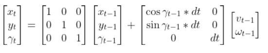
Let’s get back to our two-wheeled mobile robot. It has three states (like in the state space modeling tutorial.) The forward kinematics can be modeled as:
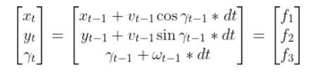
The state space model is as follows:
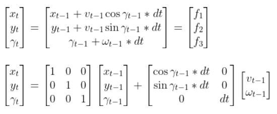
This model above shows the state of the robot at time t [x position, y position, yaw angle] given the state at time t-1, and the control inputs that were applied at time t-1.
The control inputs in this example are the linear velocity (v) — which has components in the x and y direction — and the angular velocity around the z axis, ω (also known as the “yaw rate”).
Our robot starts out at the origin (x=0 meters, y=0 meters), and the yaw angle is 0 radians. Thus the state at t-1 is:
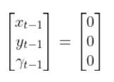
We let dt = 1 second. dt represents the interval between timesteps.
Now suppose we want our robot to drive to coordinate (x=2,y=2). This is our desired state (i.e. our goal destination).
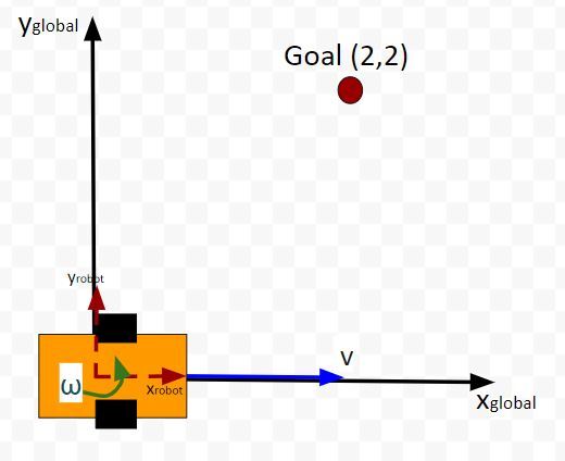
Also, we want the robot to face due north (i.e. 90 degrees (1.5708 radians) yaw angle) once it reaches the desired state. Therefore, our desired state is:
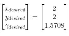
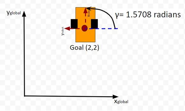
We launch our robot at time t-1, and we feed it our desired state. The robot must use the LQR algorithm to solve for the optimal control inputs that minimize both the state error and actuator effort. In other words, we want the robot to get from (x=0, y=0) to (x=2, y=2) and face due north once we get there. However, we don’t want to get there so fast so that we drain the car’s battery.
These optimal control inputs then get fed into the control input vector to predict the state at time t.
In other words, we use LQR to solve for this:

And then plug that vector into this:
to get the state at time t.
One more thing to make this simulation more realistic. Let’s assume the maximum linear velocity of the robot car is 3.0 meters per second, and the maximum angular velocity is 90 degrees per second (1.5708 radians per second).
Let’s take a look at all this in Python code.
Here is my Python implementation of the LQR. Don’t be intimidated by all the lines of code. Just go through it one step at a time. Take your time. You can copy and paste the entire thing into your favorite IDE.
Remember to play with the values along the diagonals of the Q and R matrices. You’ll see in my code that the Q matrix has been tweaked a bit.
1
2
3
4
5
6
7
8
9
10
11
12
13
14
15
16
17
18
19
20
21
22
23
24
25
26
27
28
29
30
31
32
33
34
35
36
37
38
39
40
41
42
43
44
45
46
47
48
49
50
51
52
53
54
55
56
57
58
59
60
61
62
63
64
65
66
67
68
69
70
71
72
73
74
75
76
77
78
79
80
81
82
83
84
85
86
87
88
89
90
91
92
93
94
95
96
97
98
99
100
101
102
103
104
105
106
107
108
109
110
111
112
113
114
115
116
117
118
119
120
121
122
123
124
125
126
127
128
129
130
131
132
133
134
135
136
137
138
139
140
141
142
143
144
145
146
147
148
149
150
151
152
153
154
155
156
157
158
159
160
161
162
163
164
165
166
167
168
169
170
171
172
173
174
175
176
177
178
179
180
181
182
183
184
185
186
187
188
189
190
191
192
193
194
195
196
197
198
199
200
201
202
203
204
205
206
207
208
209
210
211
212
213
214
215
216
217
218
219
220
221
222
223
224
225
226
227
|
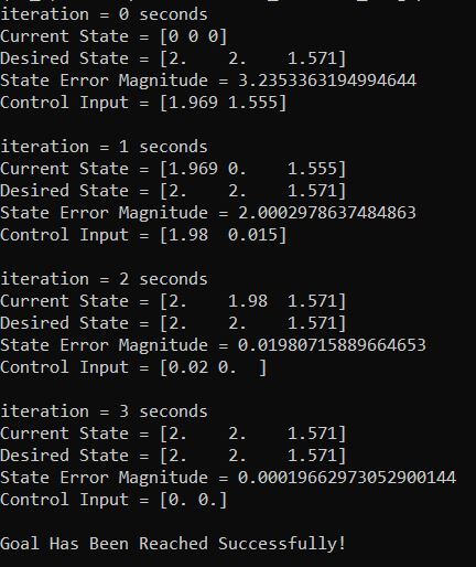
import numpy as np# Author: Addison Sears-Collins# Description: Linear Quadratic Regulator example # (two-wheeled differential drive robot car)######################## DEFINE CONSTANTS ###################################### Supress scientific notation when printing NumPy arraysnp.set_printoptions(precision=3,suppress=True)# Optional Variablesmax_linear_velocity = 3.0 # meters per secondmax_angular_velocity = 1.5708 # radians per seconddef getB(yaw, deltat): """ Calculates and returns the B matrix 3x2 matix ---> number of states x number of control inputs Expresses how the state of the system [x,y,yaw] changes from t-1 to t due to the control commands (i.e. control inputs). :param yaw: The yaw angle (rotation angle around the z axis) in radians :param deltat: The change in time from timestep t-1 to t in seconds :return: B matrix ---> 3x2 NumPy array """ B = np.array([ [np.cos(yaw)*deltat, 0], [np.sin(yaw)*deltat, 0], [0, deltat]]) return Bdef state_space_model(A, state_t_minus_1, B, control_input_t_minus_1): """ Calculates the state at time t given the state at time t-1 and the control inputs applied at time t-1 :param: A The A state transition matrix 3x3 NumPy Array :param: state_t_minus_1 The state at time t-1 3x1 NumPy Array given the state is [x,y,yaw angle] ---> [meters, meters, radians] :param: B The B state transition matrix 3x2 NumPy Array :param: control_input_t_minus_1 Optimal control inputs at time t-1 2x1 NumPy Array given the control input vector is [linear velocity of the car, angular velocity of the car] [meters per second, radians per second] :return: State estimate at time t 3x1 NumPy Array given the state is [x,y,yaw angle] ---> [meters, meters, radians] """ # These next 6 lines of code which place limits on the angular and linear # velocities of the robot car can be removed if you desire. control_input_t_minus_1[0] = np.clip(control_input_t_minus_1[0], -max_linear_velocity, max_linear_velocity) control_input_t_minus_1[1] = np.clip(control_input_t_minus_1[1], -max_angular_velocity, max_angular_velocity) state_estimate_t = (A @ state_t_minus_1) + (B @ control_input_t_minus_1) return state_estimate_t def lqr(actual_state_x, desired_state_xf, Q, R, A, B, dt): """ Discrete-time linear quadratic regulator for a nonlinear system. Compute the optimal control inputs given a nonlinear system, cost matrices, current state, and a final state. Compute the control variables that minimize the cumulative cost. Solve for P using the dynamic programming method. :param actual_state_x: The current state of the system 3x1 NumPy Array given the state is [x,y,yaw angle] ---> [meters, meters, radians] :param desired_state_xf: The desired state of the system 3x1 NumPy Array given the state is [x,y,yaw angle] ---> [meters, meters, radians] :param Q: The state cost matrix 3x3 NumPy Array :param R: The input cost matrix 2x2 NumPy Array :param dt: The size of the timestep in seconds -> float :return: u_star: Optimal action u for the current state 2x1 NumPy Array given the control input vector is [linear velocity of the car, angular velocity of the car] [meters per second, radians per second] """ # We want the system to stabilize at desired_state_xf. x_error = actual_state_x - desired_state_xf # Solutions to discrete LQR problems are obtained using the dynamic # programming method. # The optimal solution is obtained recursively, starting at the last # timestep and working backwards. # You can play with this number N = 50 # Create a list of N + 1 elements P = [None] * (N + 1) Qf = Q # LQR via Dynamic Programming P[N] = Qf # For i = N, ..., 1 for i in range(N, 0, -1): # Discrete-time Algebraic Riccati equation to calculate the optimal # state cost matrix P[i-1] = Q + A.T @ P[i] @ A - (A.T @ P[i] @ B) @ np.linalg.pinv( R + B.T @ P[i] @ B) @ (B.T @ P[i] @ A) # Create a list of N elements K = [None] * N u = [None] * N # For i = 0, ..., N - 1 for i in range(N): # Calculate the optimal feedback gain K K[i] = -np.linalg.pinv(R + B.T @ P[i+1] @ B) @ B.T @ P[i+1] @ A u[i] = K[i] @ x_error # Optimal control input is u_star u_star = u[N-1] return u_stardef main(): # Let the time interval be 1.0 seconds dt = 1.0 # Actual state # Our robot starts out at the origin (x=0 meters, y=0 meters), and # the yaw angle is 0 radians. actual_state_x = np.array([0,0,0]) # Desired state [x,y,yaw angle] # [meters, meters, radians] desired_state_xf = np.array([2.000,2.000,np.pi/2]) # A matrix # 3x3 matrix -> number of states x number of states matrix # Expresses how the state of the system [x,y,yaw] changes # from t-1 to t when no control command is executed. # Typically a robot on wheels only drives when the wheels are told to turn. # For this case, A is the identity matrix. # Note: A is sometimes F in the literature. A = np.array([ [1.0, 0, 0], [ 0,1.0, 0], [ 0, 0, 1.0]]) # R matrix # The control input cost matrix # Experiment with different R matrices # This matrix penalizes actuator effort (i.e. rotation of the # motors on the wheels that drive the linear velocity and angular velocity). # The R matrix has the same number of rows as the number of control # inputs and same number of columns as the number of # control inputs. # This matrix has positive values along the diagonal and 0s elsewhere. # We can target control inputs where we want low actuator effort # by making the corresponding value of R large. R = np.array([[0.01, 0], # Penalty for linear velocity effort [ 0, 0.01]]) # Penalty for angular velocity effort # Q matrix # The state cost matrix. # Experiment with different Q matrices. # Q helps us weigh the relative importance of each state in the # state vector (X, Y, YAW ANGLE). # Q is a square matrix that has the same number of rows as # there are states. # Q penalizes bad performance. # Q has positive values along the diagonal and zeros elsewhere. # Q enables us to target states where we want low error by making the # corresponding value of Q large. Q = np.array([[0.639, 0, 0], # Penalize X position error [0, 1.0, 0], # Penalize Y position error [0, 0, 1.0]]) # Penalize YAW ANGLE heading error # Launch the robot, and have it move to the desired goal destination for i in range(100): print(f'iteration = {i} seconds') print(f'Current State = {actual_state_x}') print(f'Desired State = {desired_state_xf}') state_error = actual_state_x - desired_state_xf state_error_magnitude = np.linalg.norm(state_error) print(f'State Error Magnitude = {state_error_magnitude}') B = getB(actual_state_x[2], dt) # LQR returns the optimal control input optimal_control_input = lqr(actual_state_x, desired_state_xf, Q, R, A, B, dt) print(f'Control Input = {optimal_control_input}') # We apply the optimal control to the robot # so we can get a new actual (estimated) state. actual_state_x = state_space_model(A, actual_state_x, B, optimal_control_input) # Stop as soon as we reach the goal # Feel free to change this threshold value. if state_error_magnitude < 0.01: print("\nGoal Has Been Reached Successfully!") break print()# Entry point for the programmain() |
You can see in the output that it took about 3 seconds for the robot to reach the goal position and orientation. The LQR algorithm did its job well.
Note that you can remove the maximum linear and angular velocity constraints if you have issues in getting the correct output. You can remove these constraints by going to the state_space_model method inside the code I pasted in the previous section.
That’s it for the fundamentals of LQR. If you ever run across LQR in the future and need a refresher, just come back to this tutorial.
Keep building!
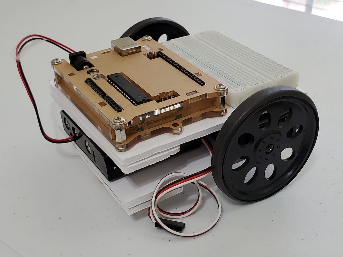
In this tutorial, we will learn how to derive the observation model for a two-wheeled mobile robot (I’ll explain what an observation model is below). Specifically, we’ll assume that our mobile robot is a differential drive robot like the one on the cover photo. A differential drive robot is one in which each wheel is driven independently from the other.
Below is a representation of a differential drive robot on a 3D coordinate plane with x, y, and z axes. The yaw angle γ represents the amount of rotation around the z axis as measured from the x axis.
Here is the aerial view:
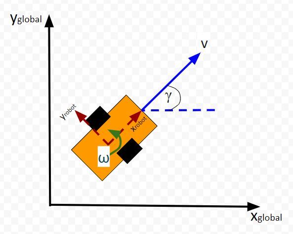
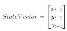
Table of Contents
Typically, when a mobile robot is moving around in the world, we gather measurements from sensors to create an estimate of the state (i.e. where the robot is located in its environment and how it is oriented relative to some axis).
An observation model does the opposite. Instead of converting sensor measurements to estimate the state, we use the state (or predicted state at the next timestep) to estimate (or predict) sensor measurements. The observation model is the mathematical equation that does this calculation.
You can understand why doing something like this is useful. Imagine you have a state space model of your mobile robot. You want the robot to move from a starting location to a goal location. In order to reach the goal location, the robot needs to know where it is located and which direction it is moving.
Suppose the robot’s sensors are really noisy, and you don’t trust its observations entirely to give you an accurate estimate of the current state. Or perhaps, all of a sudden, the sensor breaks, or generates erroneous data.
The observation model can help us in these scenarios. It enables you to predict what the sensor measurements would be at some timestep in the future.
The observation model works by first using the state model to predict the state of the robot at that next timestep and then using that state prediction to infer what the sensor measurement would be at that point in time.
You can then compute a weighted average (i.e. this is what you do during Kalman Filtering) of the predicted sensor measurements and the actual sensor observation at that timestep to create a better estimate of your state.
This is what you do when you do Kalman Filtering. You combine noisy sensor observations with predicted sensor measurements (based on your state space model) to create a near-optimal estimate of the state of a mobile robot at some time t.
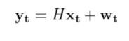
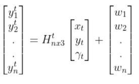
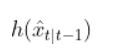
An observation model (also known as measurement model or sensor model) is a mathematical equation that represents a vector of predicted sensor measurements y at time t as a function of the state of a robotic system x at time t, plus some sensor noise (because sensors aren’t 100% perfect) at time t, denoted by vector wt.
Here is the formal equation:
Because a mobile robot in 3D space has three states [x, y, yaw angle], in vector format, the observation model above becomes:
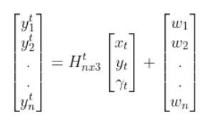
where:
Sensor observations can be anything from distance to a landmark, to GPS readings, to ultrasonic distance sensor readings, to odometry readings….pretty much any number you can read from a robotic sensor that can help give you an estimate of the robot’s state (position and orientation) in the world.
The reason why I say predicted measurements for the y vector is because they are not actual sensor measurements. Rather you are using the state of a mobile robot (i.e. the current location and orientation of a robot in 3D space) at time t-1 to predict the next state at time t, and then you use that next state (estimate) at time t to infer what the corresponding sensor measurement would be at that point in time t.
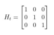
Let’s examine how to calculate H. The measurement matrix H is used to convert the predicted state estimate at time t into predicted sensor measurements at time t.
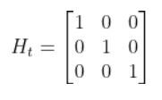
Imagine you had a sensor that could measure the x position, y position, and yaw angle (i.e. rotation angle around the z-axis) directly. What would H be?
In this case, H will be the identity matrix since the estimated state maps directly to sensor measurements [x, y, yaw].
H has the same number of rows as sensor measurements and the same number of columns as states. Here is how the matrix would look in this scenario.
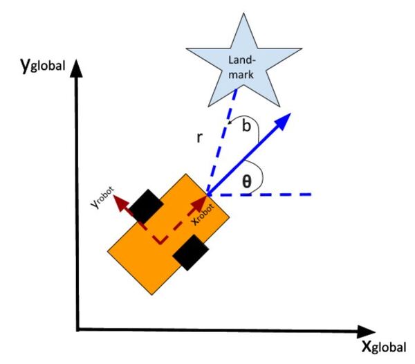
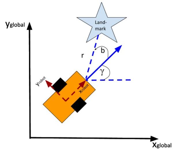
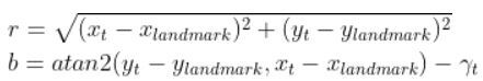
What if, for example, you had a landmark in your environment. How does the current state of the robot enable you to calculate the distance (i.e. range) to the landmark r and the bearing angle b to the landmark?
Using the Pythagorean Theorem and trigonometry, we get the following equations for the range r and bearing b:
Let’s put this in matrix form.
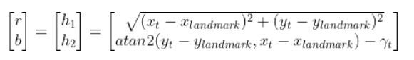
The formulas in the vector above are nonlinear (note the arctan2 function). They enable us to take the current state of the robot at time t and infer the corresponding sensor observations r and b at time t.
Let’s linearize the model to create a linear observation model of the following form:
We have to calculate the Jacobian, just as we did when we calculated the A and B matrices in the state space modeling tutorial.
The formula for Ht is as follows:
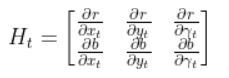
So we need to calculate 6 different partial derivatives. Here is what you should get:
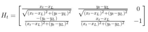
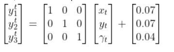
The final observation model is as follows:
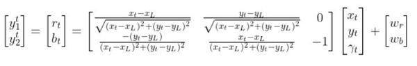
Equivalently, in some literature, you might see that all the stuff above is equal to:
In fact, in the Wikipedia Extended Kalman Filter article, they replace time t with time k (not sure why because t is a lot more intuitive, but it is what it is).
Let’s create an observation model in code. As a reminder, here is our robot model (as seen from above).

We’ll assume we have a sensor on our mobile robot that is able to give us exact measurements of the xglobal position in meters, yglobal position in meters, and yaw angle γ of the robot in radians at each timestep.
Therefore, as mentioned earlier,
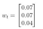
We’ll also assume that the corresponding noise (error) for our sensor readings is +/-0.07 m for the x position, +/-0.07 m for the y position, and +/-0.04 radians for the yaw angle. Therefore, here is the sensor noise vector:
So, here is our equation:
Suppose that the state of the robot at time t is [x=5.2, y=2.8, yaw angle=1.5708]. Because the yaw angle is 90 degrees (1.5708 radians), we know that the robot is heading due north relative to the global reference frame (i.e. the world or environment the robot is in).
What is the corresponding estimated sensor observation at time t given the current state of the robot at time t?
Here is the code:
1
2
3
4
5
6
7
8
9
10
11
12
13
14
15
16
17
18
19
20
21
22
23
24
25
26
27
28
29
30
31
32
33
34
35
36
37
38
|
import numpy as np# Author: Addison Sears-Collins# Description: An observation model for a differential drive mobile robot# Measurement matrix H_t# Used to convert the predicted state estimate at time t# into predicted sensor measurements at time t.# In this case, H will be the identity matrix since the # estimated state maps directly to state measurements from the # odometry data [x, y, yaw]# H has the same number of rows as sensor measurements# and same number of columns as states.H_t = np.array([ [1.0, 0, 0], [ 0,1.0, 0], [ 0, 0, 1.0]]) # Sensor noise. This is a vector with the# number of elements equal to the number of sensor measurements.sensor_noise_w_t = np.array([0.07,0.07,0.04]) # The estimated state vector at time t in the global # reference frame# [x_t, y_t, yaw_t]# [meters, meters, radians]state_estimate_t = np.array([5.2,2.8,1.5708])def main(): estimated_sensor_observation_y_t = H_t @ ( state_estimate_t) + ( sensor_noise_w_t) print(f'State at time t: {state_estimate_t}') print(f'Estimated sensor observations at time t: {estimated_sensor_observation_y_t}')main() |
Here is the output:
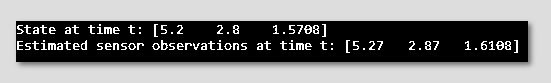
And that’s it folks. That linear observation model above enables you to convert the state at time t to estimated sensor observations at time t.
In a real robot application, we would use an Extended Kalman Filter to compute a weighted average of the estimated sensor reading using the observation model and the actual sensor reading that is mounted on your robot. In my next tutorial, I’ll show you how to implement an Extended Kalman Filter from scratch, building on the content we covered in this tutorial.
Keep building!
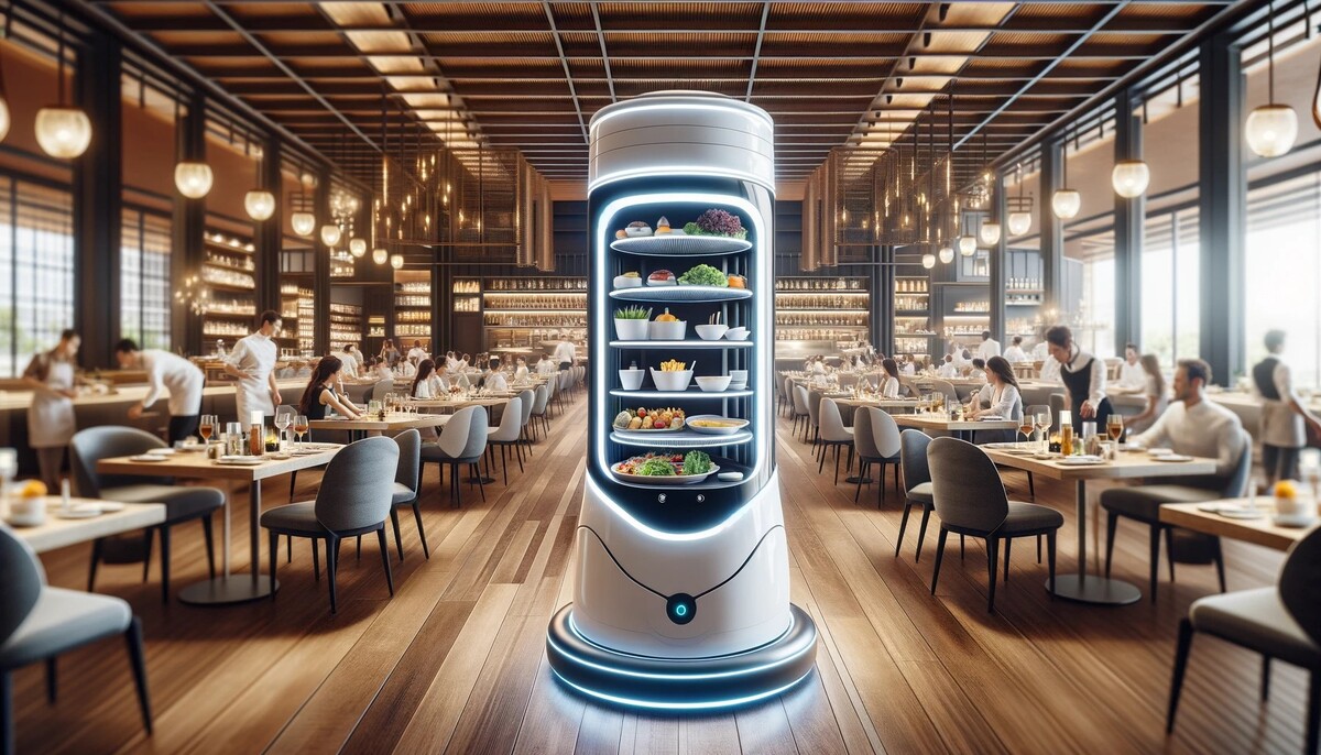
Have you ever wondered how those robots navigate around restaurants or hospitals, delivering food or fetching supplies? These little marvels of engineering often rely on a simple yet powerful concept: the differential drive robot.
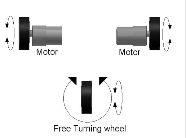
A differential drive robot uses two independently powered wheels and often has one or more passive caster wheels. By controlling the speed and direction of each wheel, the robot can move forward, backward, turn, or even spin in place.
This tutorial will delve into the behind-the-scenes calculations that translate desired robot motion (linear and angular velocities) into individual wheel speeds (rotational velocities in revolutions per second).
Table of Contents
Differential drive robots, with their two independently controlled wheels, are widely used for their maneuverability and simplicity. Here are some real-world applications:
Delivery and Warehousing:
Domestic and Public Use:
Specialized Applications:
Why Differential Drive for these Applications?
Differential drive robots offer several advantages for these tasks:
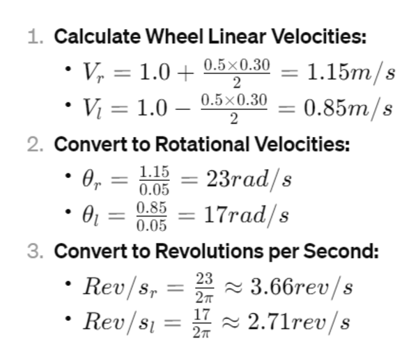
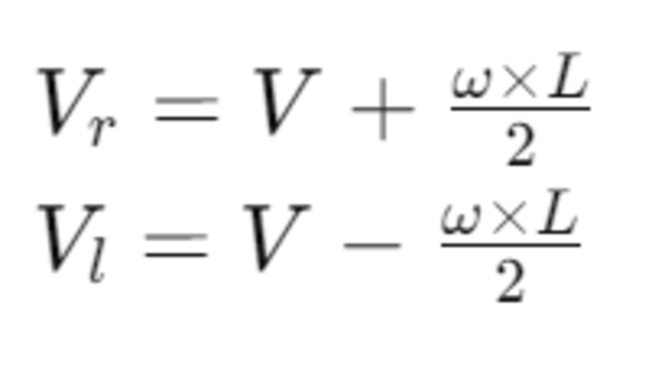
The robot’s motion is defined by two control inputs: the linear velocity (V) and the angular velocity (ω) of the robot in its reference frame.
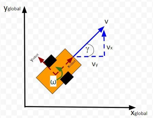
The linear velocity is the speed at which you want the robot to move forward or backward, while the angular velocity defines how fast you want the robot to turn clockwise and counterclockwise.
The linear velocities of the right (Vr) and the left (Vl) wheels can be calculated using the robot’s wheelbase width (L), which is the distance between the centers of the two wheels:
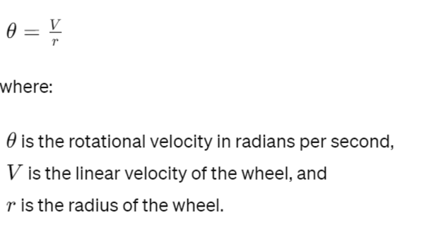
Once we have the linear velocities of the wheels, we need to convert them into rotational velocities. The rotational velocity (θ) in radians per second for each wheel is given by:
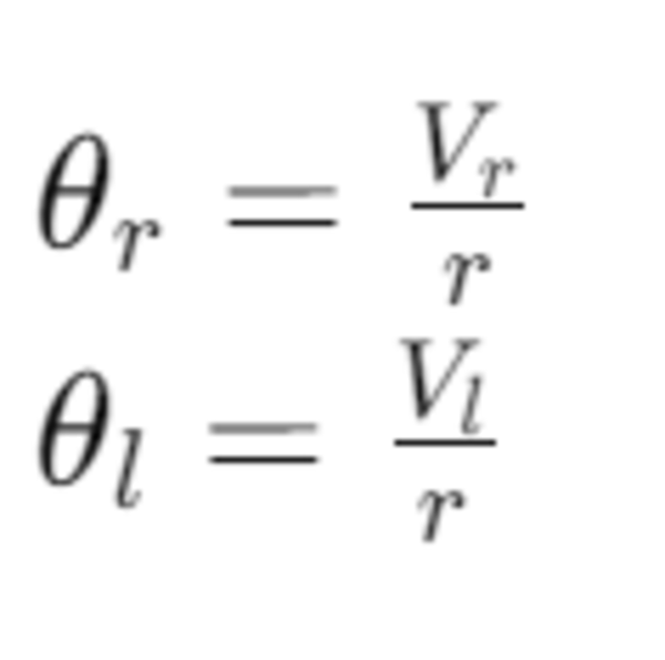
Thus, the rotational velocities of the right and left wheels are:
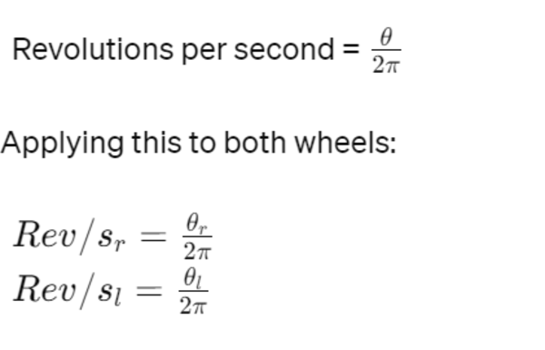
The final step is to convert the rotational velocities from radians per second to revolutions per second (rev/s) for practical use. Since there are 2π radians in a full revolution:
Let’s calculate the wheel velocities for a robot with a wheel radius of 0.05m, wheelbase width of 0.30m, commanded linear velocity of 1.0m/s, and angular velocity of 0.5rad/s.