What is RTK GPS? In fields like surveying, construction, and agriculture, precision isn’t optional—it’s essential. In many of these tasks, being off by even a few meters can lead to wasted time, costly mistakes, or failed inspections. That’s why professionals turn to high-precision positioning technologies like RTK GPS.

But to understand how RTK delivers centimeter-level results, we first need to look at the system it relies on—GNSS. GNSS provides the global coverage and satellite data that RTK builds upon. It’s the foundation of all satellite-based positioning.

Let’s start with the basics of how GNSS positioning works—and then explore how RTK takes it to the next level.

How does GNSS positioning work?

Global Navigation Satellite Systems, or GNSS, refer to satellite constellations like GPS, GLONASS, Galileo, and BeiDou. These systems provide global satellite positioning services. Many industries — from mobile navigation and logistics to construction and autonomous systems — use them in daily life.

GNSS receivers calculate their position by measuring how long it takes for signals from satellites to reach the receiver. Each signal includes data on satellite location and transmission time. When a receiver picks up signals from at least four satellites, it can determine its position on Earth.

Most standard GNSS receivers, like those in smartphones or drones, offer accuracy in the range of 2 to 4 meters. That’s fine for casual navigation, but for tasks like land surveying, construction layout, or precision agriculture, meter-level accuracy falls short.

That’s where high-precision GNSS positioning techniques like RTK come in.

What is RTK GPS?

RTK, or Real-Time Kinematic, is a positioning method that improves GNSS accuracy from meters down to centimeters. It does this by correcting satellite signal errors in real time.

An RTK system includes two GNSS receivers: a base and a rover. The base station is set at a known location and constantly receives satellite signals. It then sends corrections to the rover, which is the moving unit that needs to determine its accurate position. Because both units are observing the same satellites under nearly identical conditions, the rover can use the base’s corrections to eliminate common errors.

This method allows the rover to deliver precise position data with centimeter-level accuracy. RTK GPS technology is especially useful in surveying, mapping, agriculture, construction, and inspection tasks—where real-time precision is critical.

How RTK works?

When the rover meets the base

The base station can be a local GNSS unit or a remote reference station accessed via an RTK network. The role of the base remains the same—to provide reference data in real time that allows the rover to calculate its position with much greater accuracy.

These GNSS corrections are what make RTK stand apart from traditional GNSS. While standard GNSS relies only on signal timing, RTK takes advantage of a more detailed technique: carrier phase measurement.

Carrier phase and ambiguity resolution

GNSS signals travel as waveforms—RTK doesn’t just measure when the signal arrives, but how many full and partial wave cycles it took to get there. However, in the beginning, the receiver doesn’t know the number of whole cycles. This is called ambiguity.

RTK resolves these ambiguities by comparing signals from both base and rover. Once you resolve it, the system locks onto what’s called a FIX status—meaning the receiver has achieved centimeter-level accuracy.

This step is essential in transforming approximate GPS data into precise positioning.

Understanding RTK solution statuses

RTK solutions go through different phases as the receiver processes satellite data:

• SINGLE: No corrections are being received. Accuracy is similar to standard GNSS—several meters.
• FLOAT: Corrections have begun, but ambiguities aren’t fully resolved. Accuracy improves, but hasn’t yet reached centimeter level.
• FIX: The receiver now delivers centimeter-accurate positions after resolving ambiguities
  

Getting to FIX is the ultimate goal in any RTK setup, and maintaining FIX is key to successful high-precision work.

This video will show you how RTK technology works.

How to send RTK corrections from a base to a rover?

RTK corrections can be delivered via different channels, depending on your workflow and environment:

• Radio: Best for on-site setups without internet. It’s reliable when there’s a direct line of sight between the base and the rover.
• NTRIP: A protocol that sends corrections over the internet. Perfect for longer distances or when using a network of reference stations.
• Dual-streaming: Some systems support broadcasting over both radio and internet simultaneously. This ensures corrections stay stable even when one method becomes unreliable.

These flexible delivery methods allow users to choose the right setup for their environment—urban, rural, or remote.

What are the differences between RTK solution statuses?

RTK solutions go through different phases as the receiver processes satellite data:

• SINGLE: No corrections are being received. Accuracy is similar to standard GNSS—several meters.
• FLOAT: Corrections have begun, but ambiguities aren’t fully resolved. Accuracy improves, but hasn’t yet reached centimeter level.
• FIX: Ambiguities are resolved, and the receiver is now delivering centimeter-accurate positions.
  

Getting to FIX is the ultimate goal in any RTK setup, and maintaining FIX is key to successful high-precision work.

How to get the best RTK GPS performance in the field?

RTK depends on specific conditions to perform at its best, including but not limited to a short baseline between the base and rover, a clear view of the sky, and distance from sources of electromagnetic interference to avoid signal distortion.

Baseline

The distance between base and rover, known as the baseline, is a key factor. The closer the two units are, the more similar their satellite observations will be. Long baselines introduce environmental differences—like varying atmospheric conditions—that reduce correction effectiveness. Keeping the baseline short helps maintain the accuracy of RTK.

Satellite visibility

GNSS relies on a clear sky view. Obstacles like buildings, trees, or terrain features can block or reflect signals, weakening the quality of the data. A clear line of sight to the sky is essential for consistent fixes.

Electromagnetic interference

Electronic equipment, power lines, or heavy machinery can interfere with GNSS signals. Keeping your receiver away from such sources improves reliability and reduces signal noise.

To learn more about factors that affect signal accuracy, read our guide on eight common mistakes in GNSS surveying and how to fix them. 

Where RTK is used?

RTK GPS is now a standard tool across many industries that rely on spatial accuracy:

• Surveying and mapping: From topographic surveys to construction layout.
• Precision agriculture: Automating machinery, planting, and soil analysis with sub-inch accuracy.
• Drone mapping: Enhancing data for orthomosaics and 3D models.
• Construction: Layout tasks, volume measurement, and quality control.
• Inspection and infrastructure: Power lines, roads, pipelines, and more.

The wide range of RTK uses highlights its value in turning GNSS from a navigation tool into a precise positioning instrument. This technique transforms GNSS from a general positioning tool into a high-precision system suitable for professional tasks. RTK delivers the accuracy you need—especially when paired with the right tools, like the Emlid Reach RS3 receivers.

If you’re looking to boost efficiency, improve data quality, and unlock centimeter-level results in the field, RTK GPS is the technology to build your workflow on.

Meet the RTK GNSS lineup that makes precision look easy

Need centimeter-level accuracy but don’t want to wrestle with complicated gear, outdated workflows, or fragile equipment? Modern RTK GNSS doesn’t have to feel like a surveying textbook.

Today’s field teams—whether in construction, GIS, engineering, or mapping—need tools that remove friction, not add to it. That means fast setup, reliable all-band RTK performance, and the freedom to move without constantly leveling poles or rechecking points:

Reach RS4 Pro is our most advanced all-band RTK GNSS receiver, combining centimeter-level positioning with dual cameras, AR stakeout, image-based measurements, and tilt compensation. It’s built for teams who want to move faster on site, capture more in one go, and rethink what a GNSS rover can actually do.

Reach RS4 delivers powerful all-band RTK performance with tilt compensation in a streamlined setup—perfect for topographic surveys, design set-out, and everyday fieldwork where precision is non-negotiable.

Reach RX2 is the ultralight RTK rover made for mobility. With tilt compensation and full RTK capability, it’s ideal for GIS mapping, layout, and terrestrial scanning—high accuracy, zero bulk.

FAQs

What’s the difference between GPS and GNSS?
GNSS includes multiple satellite systems—GPS, GLONASS, Galileo, BeiDou—while GPS refers only to the American system. GNSS offers broader coverage and better reliability.

What does RTK mean in GPS?
RTK stands for Real-Time Kinematic. It’s a technique that provides high-precision positioning by correcting GNSS signals in real time.

Can I use RTK without a base station?
Yes and no. You don’t necessarily need to own your local base station. However, you need to connect to a source of corrections data. This could be CORS or a remote reference station—you can connect to it over the internet using the NTRIP protocol.

How accurate is RTK?
With proper setup, RTK provides centimeter-level accuracy—far beyond the meter-level positioning of traditional GPS.

What happens without RTK?
Without RTK, your receiver falls back to standard GNSS, which is only meter-accurate, which may not be sufficient for your surveying tasks.

1、主控

C-RTK 2 采用 STM32H7 处理器，Cortex-M7 内核（带双精度浮点单元），运行频率高达 480MHz，2MB Flash，1MB RAM

2、GNSS芯片

u-blox F9P

3、IMU芯片

高精度工业级的 ICM-20689 加速计&陀螺仪、RM3100 电子罗盘、ICP10111 气压计

这篇文章旨在提供一个具体的例子，让机器人专家们对李代数及其在机器人领域的应用有所了解。我最初学习李代数时，感觉网上关于李代数的解释过于浅显，缺乏清晰易懂的数学细节。希望这篇文章能够弥合这种差距。让我们开始吧。

按回车键或点击查看完整尺寸的图片

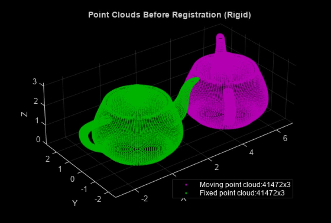
本文仅考虑迭代最近点算法（Iterative Closest Point，ICP）。为简单起见，我们仅讨论旋转问题，不涉及平移。ICP 算法通过最小化对应点之间的距离来对齐两个点云。在本例中，它优化旋转矩阵 R 以减小平方差之和。

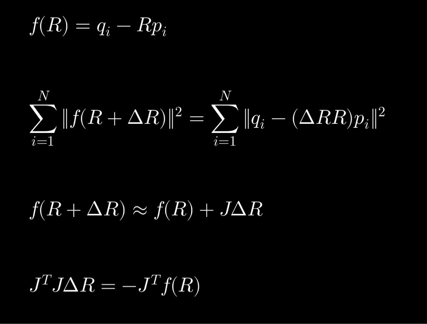
如同许多工程实践一样，我们希望使用一阶泰勒级数展开来近似函数，展开平方项，对 ΔR 求导，令导数为零，最终将问题表示为一个正规方程。求解该方程即可得到 ΔR，进而可以用它更新 R。ICP 问题正是通过多次重复此过程（假设收敛）来求解的，因此得名“迭代”。

按回车键或点击查看完整尺寸的图片

然而，这里我们遇到了一个问题。如果我们把3x3旋转矩阵看作9个独立元素并求解，结果很可能不是旋转矩阵。旋转矩阵需要满足诸如det(R)=1和RR^T=I单位矩阵之类的约束条件。而如何在满足这些约束条件的前提下建立一个可微的代价函数，这一点并不明显。

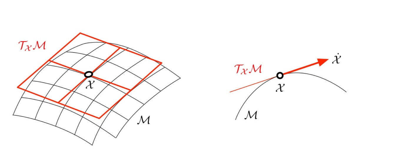
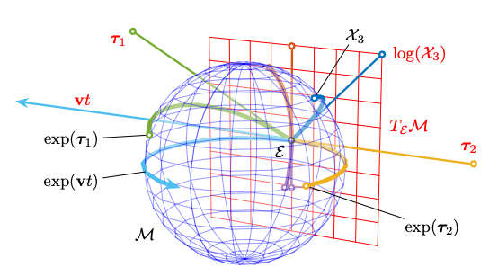
这就是李群和李代数发挥作用的地方。旋转构造属于李群，李群是一个具有流形结构的连续变换群。流形是一个光滑的广义曲面，可以局部地用线性空间（也称为切空间）逼近。这类似于地球的曲面可以局部地逼近为一个平面；虽然地球是一个三维球体，但其表面在任何一点都感觉像是一个二维平面。

按回车键或点击查看完整尺寸的图片

关键在于切空间是线性的，而李代数能够局部地捕捉这种线性结构。如果我们能够以某种方式用李代数（具有3个自由度）来表达我们的目标函数，从而将其置于线性空间中，我们就可以（再次）构建一个优化问题，而无需考虑应用于旋转矩阵的约束。

按回车键或点击查看完整尺寸的图片

这里值得稍作停顿。为什么我们用不同的数学结构来表达最初的问题后，就不再需要担心旋转矩阵的约束了呢？这是因为这些约束是由流形或李群本身施加的。

想象一下等离子体被限制在球面上，例如地球磁层上的带电粒子。如果我们想求解它们的“流体动力学”，就无法在开放域（三维空间）中进行求解。解被限制在三维空间中的一个二维曲面上。因此，如果我们用 S²（代表球面的流形）来表达这个问题，那么问题本身就是有约束的。

类似地，我们可以想象三维旋转被限制在一个具有更复杂结构的三维几何曲面（位于九维空间中）上——即李群——形式上称为特殊正交群SO(3)。该群不仅具有流形结构，而且还具有一个光滑的群运算，该运算定义了旋转如何组合。

按回车键或点击查看完整尺寸的图片

我们之前没有讨论过的一点是，李代数被定义为李群单位元处的切空间。了解这一点可以简化我们的方程，如下所示：

按回车键或点击查看完整尺寸的图片

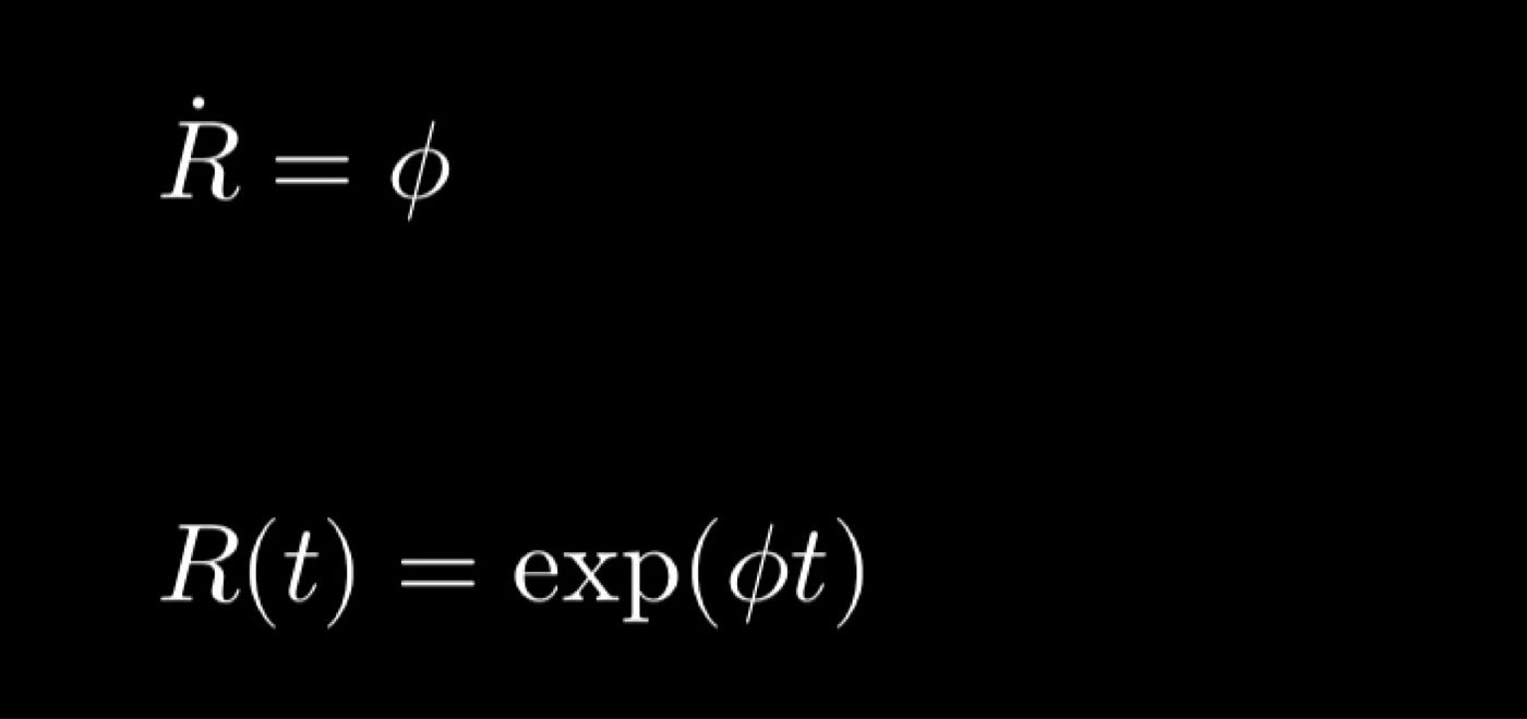
由于 R 属于李群 SO(3)，其导数 Ṙ 位于 R 的切空间中。由此我们可以推断，phi 是属于李代数 so(3) 的斜对称矩阵，即 SO(3) 在单位元处的切空间。

还记得我们希望用 3x1 向量而不是 3x3 矩阵来表示旋转（及其增量）吗？不难看出，3x1 向量和相应的反对称矩阵之间存在一一对应的关系。

我们可以将向量到反对称矩阵的转换定义为帽子符号 (∧)，反向转换定义为三角符号 (∨)。那么我们知道函数 g() 具有 exp(. ∧) 的形式，它将一个 3x1 的向量映射到一个 3x3 的旋转矩阵。

按回车键或点击查看完整尺寸的图片

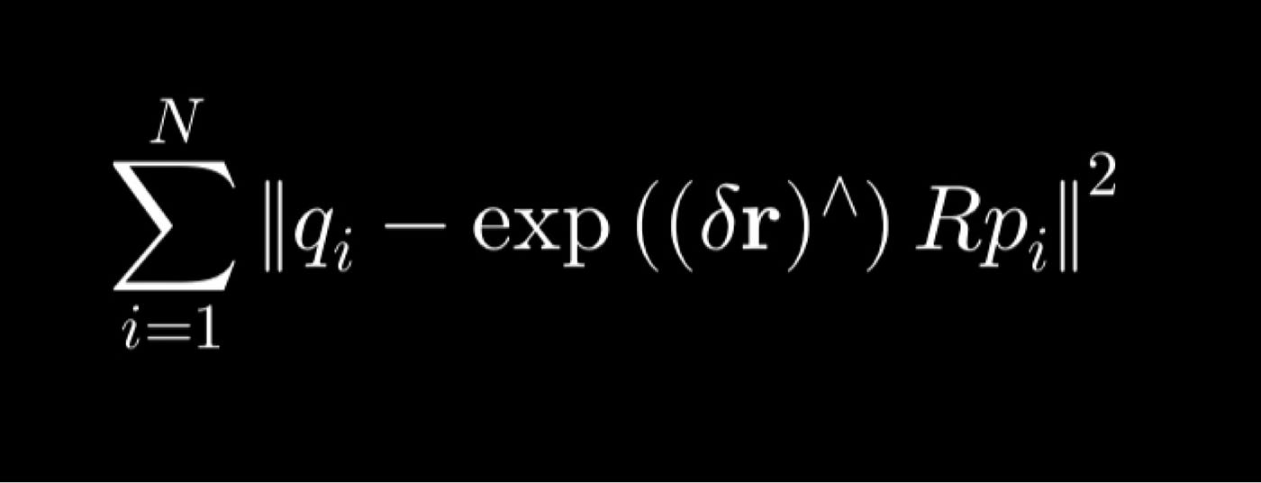
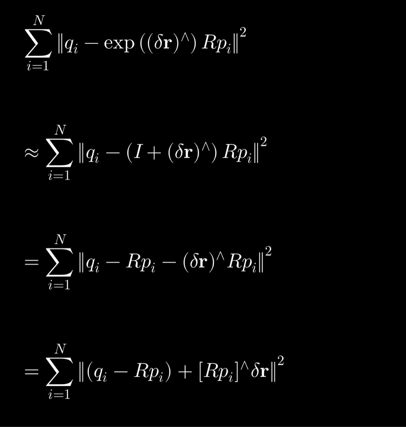
记住矩阵指数 exp(A) 可以近似为 I + A，并回想 a^b = -a^b，其中 a^b 可以理解为两个 3x1 向量 a 和 b 的叉积。然后我们最终可以将代价函数表示为 f(R + δr) ≈ f(R) + Jδr，其中 J 等于 [Rp]^。在求解 δr 的正规方程后，我们可以更新 R ← exp(δr) R。

按回车键或点击查看完整尺寸的图片

本文到此结束。当然，还有其他更直观的方法可以解决ICP问题。但在诸如扩展卡尔曼滤波（EKF）或同步定位与建图（SLAM）等应用中，由于涉及将三维旋转作为状态向量，推导雅可比矩阵并用李代数表示协方差会很有帮助。

李群既是流形又是群，其群运算——乘法和逆运算——是光滑（无限可微）映射。换句话说，它无缝地融合了代数结构（来自群论）和几何结构（来自流形）。这种几何框架自然地与线性代数和工程数学相结合，为分析连续变换（例如旋转和刚体运动）提供了强大的工具。

如需进一步阅读，我推荐阅读“用于机器人状态估计的微观李理论”。