The Extended Kalman Filter is a special Kalman Filter used when working with nonlinear systems. Since the Kalman Filter can not be applied to nonlinear systems, the Extended Kalman Filter was created to solve that problem. Specifically, it was used in the development of navigation control systems aboard Apollo 11. And like many other real world systems, the behavior is not linear so a traditional Kalman Filter can not be used. This post will walk you through an Extended Kalman Filter Python example so you can see how one can be implemented!

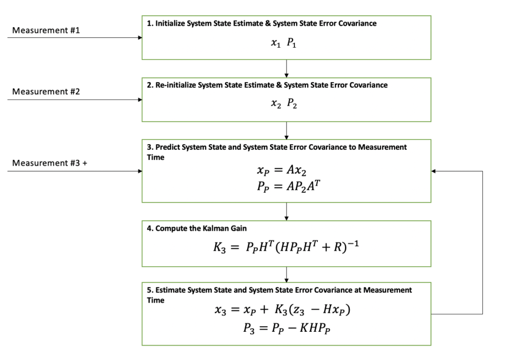
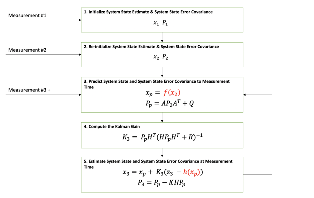
In the diagram below, it can be seen that the Extended Kalman Filter’s general flow is exactly the same as the Kalman Filter. The main two differences between the Kalman Filter and the Extended Kalman Filter are represented in red font. In addition to these differences, there are some lower level differences that I will cover in more detail below.

This article assumes that the reader understands the core concepts of the Kalman Filter. If you want a refresher before reading on, try skimming my Kalman Filter Explained Simply article.

Python Example Overview

The Extended Kalman Filter Python example chosen for this article takes in measurements from a ground based radar tracking a ship in a harbor and estimates the ships position and velocity. The radar measurements are in a local polar coordinate frame and the filter’s state estimate is in a local cartesian coordinate frame. The measurement to state estimate relationship i.e. polar to cartesian is nonlinear.

In this example, the ship is traveling in a straight line at constant velocity of 20 meters/sec or about 45 miles per hour. It is located about 3250 meters away or about 2 miles. The measurements are being reported at 1 hertz or once per second. The measurements are being reported as the range and azimuth values in local polar frame and input measurement data can be seen in the two plots below.

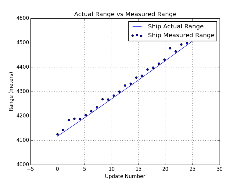
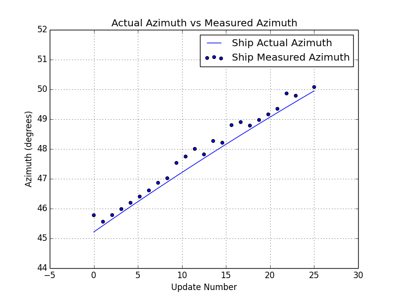
A simulation technique was used to generate these measurements. The code for simulating this ship behavior is beyond the scope of this post, but the plots above show the noisy measurements that are based on simulated position data.

On the Initialization of the Extended Kalman Filter

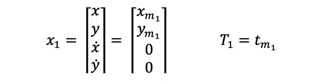
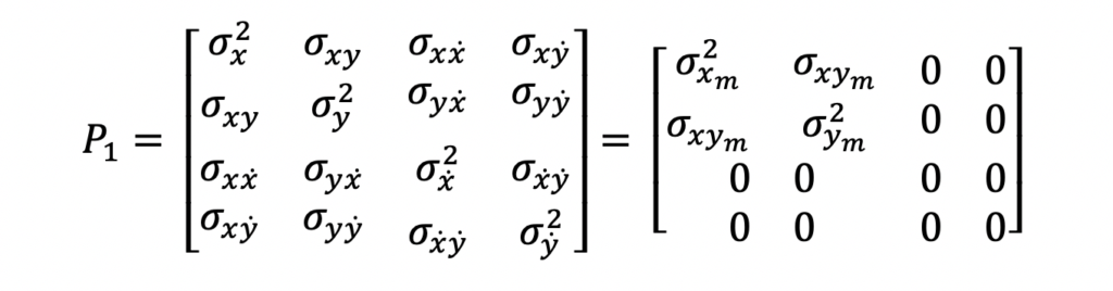
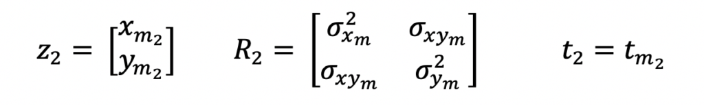
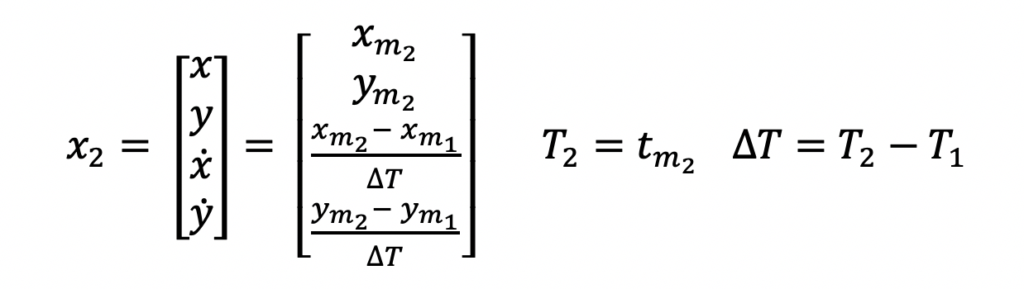
As can be seen in the Extended Kalman Filter diagram above, the first two measurements are needed before filtering can be begin. The reason for this is because the output state estimate needs to be initialized. There are different approaches to filter initialization based on your application but for this example, the first two position measurements will be used to form the state estimate which consists of the position and velocity.

Logically, one can make sense of this. The first position measurement received only tells you about the ships position at one point in time. Only after you receive the second measurement, can you compute a velocity i.e. change in position measurement divided by the time difference between the two measurements.

Extended Kalman Filter Python Example

Let’s take a look at the input, output, and system model equations before we dive into the code. This should make reading the code much easier.

Input and Output Equations

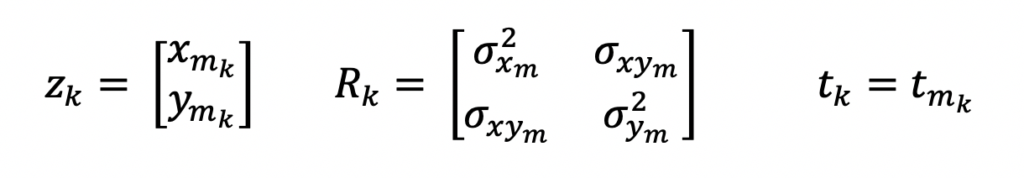
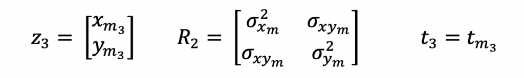
As mentioned above, the input measurements for this Extended Kalman Filter Python example are in the local polar coordinate frame. And these are the equations that represent these measurements.

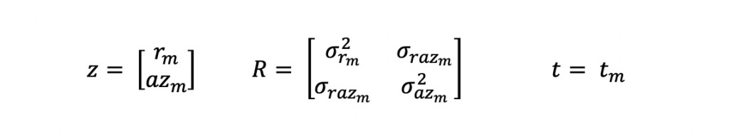
z is the measurement vector, R is the measurement covariance matrix and t is the time at which the measurement was taken. m is used as a subscript to indicate measurements.

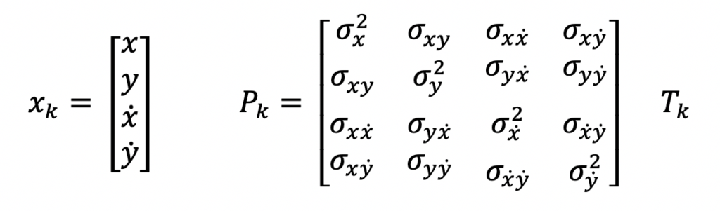
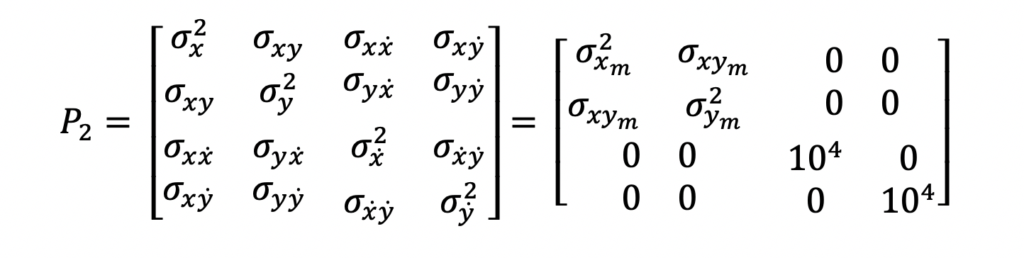
The above input measurements are filtered and a system state estimate is computed and output in the following form.

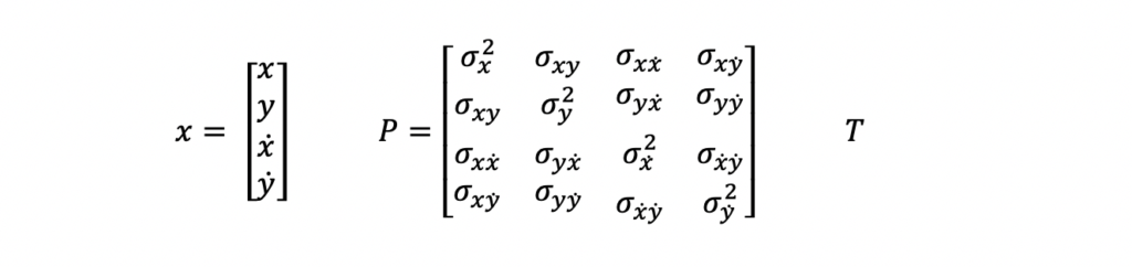
x is the state vector, P is the state covariance matrix, and T is the time at which the state estimate is valid. In this example, this time will reflect the last measurement time that was used to compute the state estimate.

System Model Equations for Prediction Step

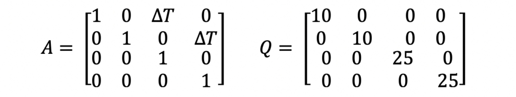
As mentioned above, the system model equations are where the primary differences between the Extended Kalman Filter and the traditional Kalman Filter lie. For this example, the A and Q matrices used are not any different than matrices that would be used in a Kalman Filter. Those equations are the following.

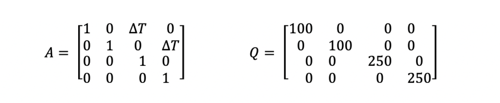
The A matrix above is the state transition matrix. This matrix is used to extrapolate the state vector and state covariance from the last data time to align with the data time of the new measurement. This matrix was developed assuming the ship was traveling linearly at constant velocity i.e. using physics equations of motion.

The Q matrix is the system noise matrix. This represents the uncertainty in the system prediction model. For this example, the A matrix assumes the ship is traveling in a linear motion at a constant velocity. But in reality, this is not always true. The Q matrix is used to add error to the state estimate prediction to account for those differences in linear motion and small accelerations or decelerations. The values used in this example are not optimized. Optimization of these parameters is outside the scope of this post.

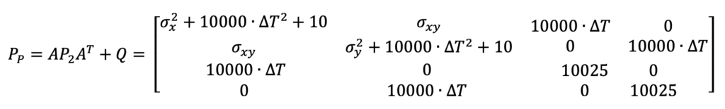
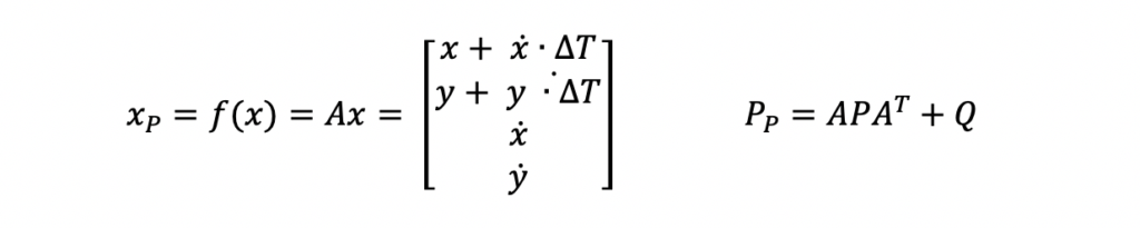
Here are the prediction equations from Step 3 in the diagram above.

System Model Equations for Estimation Step

The estimation process for the Extended Kalman Filter is performed in two steps. First, the Kalman Gain is computed. Second, the state vector and state covariance for the new measurement time is computed with the Kalman Gain. Both of these steps require the use of an H matrix. The H matrix is the state-to-measurement transition matrix. This matrix is used to transform the predicted state vector and covariance matrix into the same form as the input measurement. For this Extended Kalman Filter example, the state and measurement relationship is nonlinear. Because of this nonlinear relationship, the H matrix is different than that of a traditional Kalman Filter. Specifically, the H matrix is a jacobian matrix. The derivation and applications of the jacobian matrix are outside the scope of this post. The important features to note about the jacobian at this time is that is made up of first order partial differential equations. Here is the H matrix for this example.

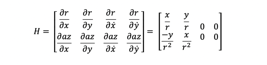
The partial differential equations were computed with the following polar to cartesian relationships for range and azimuth.

After the H matrix is computed, the Kalman Gain can be computed. The Kalman Gain equations that follow consist of two steps. First, compute the innovation matrix, S. Then compute the gain, K.

The estimation steps use the Kalman Gain, K. The estimation steps include estimating the new system state as well as the associated state covariance matrix. One difference you can see in these equations compared to the traditional Kalman Filter estimation equations, is the h(x_P) function. This function represents the state-to-measurement nonlinear transformation.

h(x_P) is defined by the equation below for this example. These equations should look familiar because these are the same equations used to compute the jacobian H matrix.

Our Extended Kalman Filter tutorial is implemented in Python with these equations. Next, we will review the implementation details with code snippets and comments.

Python Implementation for the Extended Kalman Filter Example

In order to develop and tune a Python Extended Kalman Filter, you need the following source code functionality:

• Input measurement data (real or simulated)
• Extended Kalman Filter algorithm
• Data collection and visualization tools
• Test code to read in measurement data, execute filter logic, collect data, and plot the collected data

For this tutorial, multiple Python libraries are used to accomplish the above functionality. The NumPy Python library is used for arrays, matrices, and linear algebra operations on those structures. The Matplotlib is used to plot input and output data. Assuming these packages are installed, this is the code used to import and assign a variable name to these packages.

Extended Kalman Filter Algorithm

The algorithm is implemented using one function with two input arguments, the measurement data structure, z, and the update number, updateNumber. The update number is not a necessary input variable. But for this example, it was easier to implement. Additionally, the update number was used as the time stamp for each measurement because the measurements were reported once a second. I will update this in the future to be more robust.

There are three main processing threads through this function determined by the update number: initialization, re-initialization, and filtering. Here is the code:

Testing the Extended Kalman Filter Algorithm

In order to test this algorithm implementation, real data or simulated data is needed. For this tutorial, simulated data is generated and used to test the algorithm. As mentioned above, the simulation for this example is outside the scope of this post.

The test code below was used to test this algorithm. The getMeasurements() function returns an array of arrays of measurement information in the following form: [measurement_range, meas_azimuth, measurement_cov, meas_time]

Filter Results and Analysis

There are many different ways to analyze your filter’s performance. And every application will require different analysis because each will have its own performance requirements. Here are two plots that helped us understand if this filter was working.

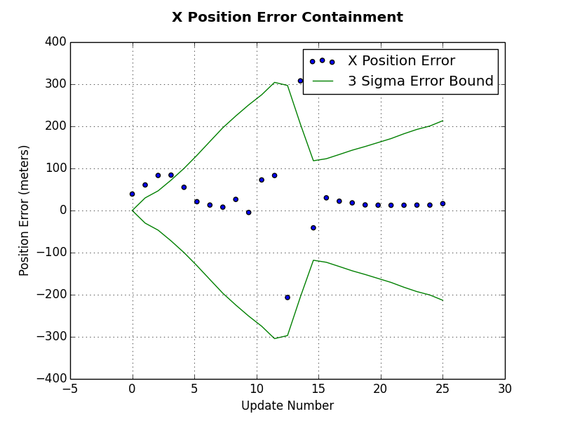
The first plot is an error plot for the x position estimate. This plot includes the x position error, which is computed as the x position estimate minus the real x position that was used to generate the polar measurement. In addition to the x position error, the green lines represent the estimated error bounds computed from the state covariance estimate. You can see in this plot that sometimes the x position error falls outside the error bounds. Again, based on your application requirements, this may or may not be okay. The x position error starts to settle within the error bounds after update number 15.

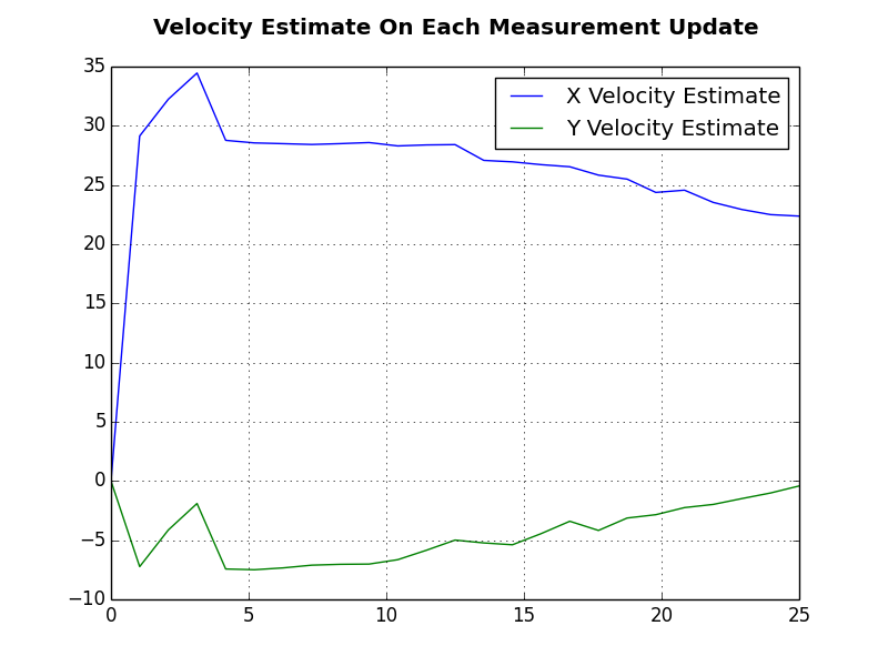
Another plot used was the estimated velocity for the ship. It can be seen that the x and y velocity values vary during the first few updates but then begin to settle at the actual values used for measurement generation i.e. x velocity at 20 meters per second and y velocity at 0 meters per second. This is a good sign that the filter is working because it is able to accurately estimate the ships velocity based only on position measurements in a different coordinate frame.

Extended Kalman Filters can diverge. This means that the filter’s estimate will grow uncontrollably and won’t represent the true system state. Researchers continue to conduct research to find ways to correct that divergence. Divergence correction is outside the scope of this post.

Summary

I wish you the best of luck in your filtering work as you move forward on your projects! Please leave a comment if you enjoyed this post!

The truth is, anybody can understand the Kalman Filter if it is explained in small digestible chunks. This post simply explains the Kalman Filter and how it works to estimate the state of a system.

The big picture of the Kalman Filter

Lets look at the Kalman Filter as a black box. The Kalman Filter has inputs and outputs. The inputs are noisy and sometimes inaccurate measurements. The outputs are less noisy and sometimes more accurate estimates. The estimates can be system state parameters that were not measured or observed. This last sentence describes the super power of the Kalman Filter. Again, the Kalman Filter estimates system parameters that are not observed or measured.

In short, you can think of the Kalman Filter as an algorithm that can estimate observable and unobservable parameters with great accuracy in real-time. Estimates with high accuracy are used to make precise predictions and decisions. For these reasons, Kalman Filters are used in robotics and real-time systems that need reliable information.

What is the Kalman Filter?

Simply put, the Kalman Filter is a generic algorithm that is used to estimate system parameters. It can use inaccurate or noisy measurements to estimate the state of that variable or another unobservable variable with greater accuracy. For example, Kalman Filtering is used to do the following:

• Object Tracking – Use the measured position of an object to more accurately estimate the position and velocity of that object.
• Body Weight Estimate on Digital Scale – Use the measured pressure on a surface to estimate the weight of object on that surface.
• Guidance, Navigation, and Control – Use Inertial Measurement Unit (IMU) sensors to estimate an objects location, velocity, and acceleration; and use those estimates to control the objects next moves.

The real power of the Kalman Filter is not smoothing measurements. It is the ability to estimate system parameters that can not be measured or observed with accuracy. Estimates with improved accuracy in systems that operate in real time, allow systems greater control and thus more capabilities.

Kalman Filter Algorithm Overview

The process diagram above shows the Kalman Filter algorithm step by step. I know those equations are intimidating but I assure you this will all make sense by the time you finish reading this article. Let’s look at this process one step at a time. For your reference, here is a table of definitions that will be referred to throughout.

The table above identifies the variables used in the algorithm. Each variable listed has a structure type and category. As this article continues, use the table as a reference.

Kalman Filter Radar Tracking Tutorial

This tutorial will go through the step by step process of a Kalman Filter being used to track airplanes and objects near airports. The output track states are used to display to the air traffic control operators monitoring the air space.

Kalman Filter Tutorial Notation

Radars are not built equally. Each one has different capabilities and therefore provides different types of information to its supporting systems. For this example, the radar will output its measurements in 2D cartesian coordinates, x and y. These measurements will be represented as a 2-by-1 column vector, z. The associated variance-covariance matrix for these measurements, R, will also be provided by the radar along with the time tag for when the measurement occurred, t. The subscript m denotes the measurement parameters. And the k subscript denotes the order of the measurement.

The Kalman Filter estimates the objects position and velocity based on the radar measurements. The estimate is represented by a 4-by-1 column vector, x. It’s associated variance-covariance matrix for the estimate is represented by a 4-by-4 matrix, P. Additionally, the state estimate has a time tag denoted as T.

Step 1: Initialize System State

Initializing the system state of a Kalman Filter varies across applications. In this tutorial, the Kalman Filter initializes the system state with the first measurement.

In this radar tracking example, the input measurements contain position only information. The output system state will contain the position and velocity of the object.

When the first measurement comes, the only information known about the object is the position at that point in time. The system state estimate will be set to the input position after the first estimate. The system state error covariance will be set to the first measurement’s position accuracy.

Initialize System State in Equations

These equations show the input and output values for this Kalman Filter after receiving the first measurement.

Step 2: Reinitialize System State

The system state estimate is reinitialized because a velocity estimate needs a second position measurement for computation.

Velocity is estimated with a linear approximation. As you most likely recall from high school physics, velocity is equal to the distance traveled divided by the time it took to travel that distance.

The updated system state estimate will be the second measurement’s position and the computed velocity. The updated system state error covariance will be the second measurement’s position accuracy and an approximated velocity accuracy. Note that this velocity accuracy approximation is something that can be tuned and adjusted after running data through your filter. There are different ways of approximating these values so if this doesn’t match your approximation, that’s okay!

Reinitialize System State in Equations for the Kalman Filter

These equations show the input and output values for this Kalman Filter after receiving the second measurement. Note the velocity variance terms in the state covariance matrix. These values are being set to 10⁴. In other words, this value indicates a large uncertainty for the velocity state values. In this example, the velocity units are meters per second.

Quick Note on Initialization

Steps 1 and 2 used the first couple measurements to initialize and re-initialize the system estimate. Each application of the Kalman Filter may do this differently but the goal is to have a system state estimate that can be updated for future measurement with the Kalman Filter equations.

Steps 3 through 6 demonstrate how measurements are filtered in and the state estimate is updated.

Step 3: Predict System State Estimate

When the third measurement is received, the system state estimate is propagated forward to time align it with the measurement. This alignment is done so that the measurement and state estimate can be combined.

The system model is used to perform this prediction. In this example, a constant velocity linear motion model is used to approximate the objects position change over a time interval. Note that a constant velocity model does assume zero acceleration. Remember this because it will resurface later.

The constant velocity linear motion model is something you may also remember from your high school physics class. The equation states that the position of an object is equal to its initial position plus its displacement over a specified time period assuming a constant velocity.

A state transition matrix represents these equations. This matrix is used to propagate the state estimate and state error covariance matrix appropriately. You may be wondering why the state error covariance matrix is propagated. The reason for this is because when a state estimate is propagated in time, the uncertainty about its state at this future time step is inherently uncertain, so the error covariance grows.

On the Q Matrix

The Q matrix represents process noise for the system model. The system model is an approximation. Throughout the life of a system state, that system model fluctuates in its accuracy. Therefore, the Q matrix is used to represent this uncertainty and adds to the existing noise on the state. For this example, the systems actual accelerations and decelerations contribute to this error.

On the H Matrix

The Kalman Filter uses the state-to-measurement matrix, H, to convert the system state estimate from the state space to the measurement space. For some applications, this is a matrix of zeros and ones. For other applications that use the Extended Kalman Filter, the H matrix is populated with differential equations. To learn more about Extended Kalman Filters, check out my article on them here.

In this tutorial, the H matrix is a simple matrix that is set up to reduce the state estimate and error covariance to position only values rather than position and velocity.

Predict System State in Equations

Step 4: Compute the Kalman Gain

This concept is the root of the Kalman Filter algorithm and why it works. It can recognize how to properly weight its current estimate and the new measurement information to form an optimal estimate.

Step 5: Estimate System State and System State Error Covariance Matrix

The Kalman Filter uses the Kalman Gain to estimate the system state and error covariance matrix for the time of the input measurement. After the Kalman Gain is computed, it is used to weight the measurement appropriately in two computations.

The first computation is the new system state estimate. The second computation is the system state error covariance.

The state estimate computed above is the only state history the Kalman Filter retains. As a result, Kalman Filters can be implemented on machines with low memory restrictions.

Next Steps

I hope this post allowed you to see how amazing the Kalman Filter is. And when it is broken up into parts, it is not that intimidating.

In conclusion, the Kalman Filter is a generic process for optimal state estimation. It is used in a variety of applications that require accurate estimation. So now that you know what it is and how it works, go out and use it in your projects!

If you enjoyed reading this post, please share it with your friends on your favorite social network! Thanks for reading!